
Lecture
Это продолжение увлекательной статьи про электрическое поле в вакууме.
...
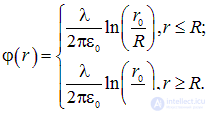
requirement of continuity of the potential at  , and the normalization
  lead to the following dependence of the potential on the distance to the axis of the cylindrical surface:
|
|
(1.52) |
In this case, when a charge infinitely large in magnitude is distributed over an infinitely long cylinder, this belongs to those cases where normalization to zero at infinity is devoid of meaning. As can be seen from (1.52), the dependence of the potential on the distance to the axis is logarithmic; normalization to zero at infinity, in the language of formula (1.52), means that  , but then the potential would be infinitely large in magnitude at any finite distance from the axis of the charged surface, which is meaningless. Choosing that finite distance
  from the axis of symmetry at which it is convenient to take the potential as equal to zero presents no difficulty and is dictated by the specifics of the problem. For example, nothing prevents us from setting
  , in which case the potential everywhere inside and on the charged surface itself will equal zero.
Let the surface charge density equal  . Such a distribution of charge over an infinite plane is characterized by the fact that its form does not depend on: a) rotation through any angle about any axis perpendicular to the plane, b) a shift by any distance along a straight line lying in the plane, in any direction. Finally, c) reflecting this charge distribution in a mirror coinciding with the plane itself leaves it unchanged.
From the symmetry analysis it is fairly obvious that the potential at any point outside the plane can depend only on the distance from that point to the plane. Let us direct the axis  of a Cartesian coordinate system perpendicular to the plane, and let the axes
  and
and  belong to the plane itself, then
|
|
(1.53) |
Moreover, by virtue of mirror symmetry, the field «in front of» the plane differs from the field «behind» the plane only in the direction of the vector  . This means that the dependence of
  on
on  must be odd, while the dependence of the potential
  on
on  must be even.
For these reasons, let us take a closed surface — the one for which we will write Gauss's theorem — of the following form (Fig. 1.51).
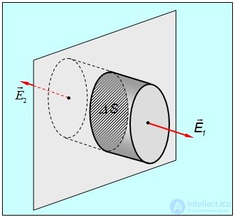
Fig. 1.51. Electric field of a charged plane
This is a cylinder with a lateral surface perpendicular to the plane and with bases parallel to the plane. The height of the cylinder is  , the area of the bases is
  . Taking into account the oddness of the dependence
  , it is convenient to place the bases of the cylinder at the same distance from the plane, so that the contribution of the bases to the flux is the same. The field strength at the bases, firstly, is perpendicular to them, secondly, is codirected with the outward normal, and thirdly, is the same in absolute value at all points of the bases
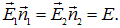
The contribution to the flux of the vector  from the lateral surface is equal to zero, since on the lateral surface
  .
.
Therefore, the total flux through the entire closed cylindrical surface is equal to
|
|
(1.54) |
Inside the cylindrical surface under consideration there is a charge

where  — is the charge density on the plane. By Gauss's theorem
 ,
,
consequently, the magnitude of the field strength of a charged plane is equal to

Let us emphasize that the result obviously does not depend on the distance from the plane at which the bases of the considered cylinder are located. It follows that on each side of the plane, the electric field it creates is uniform.
Using the previously introduced axis  perpendicular to the charged plane, the field on both sides of the plane can be described by a single formula, valid for any sign of the charge on the plane
|
|
(1.55) |
Here  — is the unit vector of the axis
  .
.
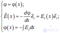
Integrating, taking into account
 ,
,
for the dependence on  of the potential of the plane's field it is easy to obtain:
|
|
(1.56) |
The potential is normalized by the condition  . Here, as in the example with an infinitely long charged cylindrical surface, the potential grows without bound as the distance goes to infinity, so normalization to zero at infinity is meaningless.
The field lines of a charged plane are shown in Fig. 1.52 and 1.53.
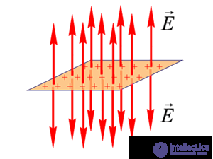
Fig. 1.52. Field of a positively charged plane
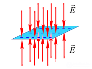
Fig. 1.53. Field of a negatively charged plane
Field of a parallel-plate capacitor
Let us determine the field strength created by two infinite parallel planes, charged uniformly and with opposite signs. The charge densities on the planes are equal in absolute value and are, respectively:  and
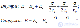
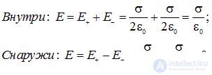
and  (an ideal parallel-plate capacitor). With the help of Fig. 1.54 it is easy to see that in the gap between the planes, the fields created by them are directed the same way, so inside, the total field is twice the field from each of the planes. Outside the planes, the fields created by them are directed in opposite directions, so the total field from both planes is equal to zero (Fig. 1.55).
|
|
(1.57) |
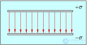
Fig. 1.54. Electric field of a parallel-plate capacitor
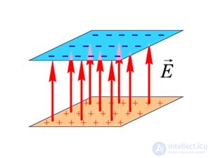
Fig. 1.55. Electric field of oppositely charged planes
|
|
(1.58) |
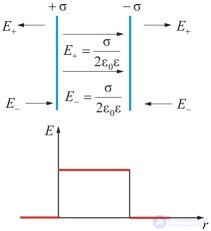
Fig. 1.56. Electric field strength of oppositely charged planes
In Appendix 6, an example is worked out involving the motion of a charged particle in a constant electric field.
As has already been noted more than once, knowing the potential of the field of a point charge and using the superposition principle, it is in principle always possible to calculate the potential of the field created by any distribution of charges.
Let us find, as an example, the potential of the electric field created on the axis of a thin disk of radius R, uniformly charged with a surface charge density (Fig. 1.57). By virtue of axial symmetry, at points on the axis the two components of the field strength perpendicular to the axis are equal to zero:  , it remains to find
  — the component of the field directed along the axis.
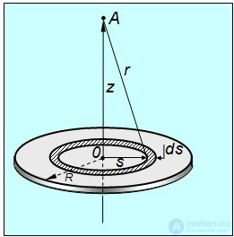
Fig. 1.57. Calculation of the potential on the axis of a charged disk
Let us select on the disk a ring of radius s and width ds (shown hatched in Fig. 1.57). The area of the ring is equal to  and therefore the charge concentrated on it is

Since all elements of the ring are at the same distance

from the observation point A, the potential  , created by the ring at point A, is given by the same formula with
  replaced by
  :
:
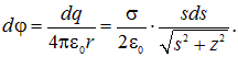
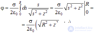
The total potential of the field, created by the entire disk at point A, is equal to the sum of the potentials from all possible rings with radii s, where 0 < s < R
|
|
(1.59) |
At large distances from the center of the disk  the square root
  can be expanded in a series, limiting to the first two terms of the expansion
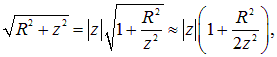
then the formula simplifies and, as it should, turns into the formula for the potential of a point charge
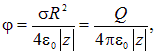
where  — is the total charge of the disk

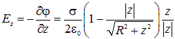
Using the relation between the field strength and the potential  , one can find the field strength on the axis of the disk
|
|
(1.60) |
The space in which we live has three dimensions. In other words, three coordinates are needed (for example,  in Cartesian or
  in spherical systems) to specify the position of a point A (Fig. 1.58). It turns out that the number 3 is closely related to the form of Coulomb's law. We have seen that the Ostrogradsky—Gauss theorem follows from Coulomb's law. The converse is also true: Coulomb's law can be derived from the Ostrogradsky—Gauss theorem. But this theorem is more general in character than Coulomb's law. In particular, it applies to spaces of dimensionality
  , where need not necessarily be equal to three.
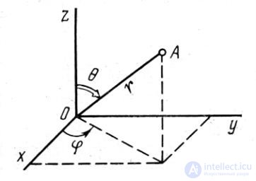
Fig. 1.58. Cartesian and spherical coordinate systems
Indeed, the theorem essentially asserts that field lines begin and end on charges or go off to infinity. The dimensionality of space plays no role here. So let us assume that we live in a space of some dimensionality and see what physics would look like in this strange world. Let us take a point charge and mentally surround it with a sphere of radius  Before continuing our acquaintance with
  -dimensional physics, let us agree on terminology.
The volume of the sphere will be measured in units of  , similar to how in our world we measure volume in
  . Thus, in two-dimensional space the role of volume is played by our area. Indeed, a sphere is the locus of points in space equidistant from the center. According to this definition, a two-dimensional sphere is a circle of radius
  two-dimensional beings would consider its volume to be what we perceive as the area of a disk
  In this section we will call the volume of a sphere in
  -dimensional space the quantity proportional to
  Similarly, the surface area of a -dimensional sphere is proportional to
  In two-dimensional space this is the length of the circle
  and it is precisely this that two-dimensional beings would perceive as surface area. On the other hand, surface area in a four-dimensional world is our three-dimensional volume.
So, the area of the sphere in an  -dimensional world is proportional to
  (the proportionality coefficient is not important to us now). The flux of the electric field strength vector in such a world is proportional to
  and must also be proportional to the magnitude of the electric charge inside the sphere (the Ostrogradsky—Gauss theorem). From this we obtain that
|
|
(10.49) |
where  — is some proportionality coefficient. An analogous expression is valid for the gravitational field in an -dimensional world.
At  we obtain from this the inverse-square law
  (Coulomb's law). At
  we find
  In fact, we are already familiar with such behavior of the electric field. It is precisely this law (10.17) that we derived for the field of an infinite charged cylinder. If one thinks it through and recalls the arrangement of the field lines of the cylinder, it becomes clear that nothing depends on the coordinate along the axis of the cylinder. Thus, this system imitates an electric field in a two-dimensional world. Now it is easier to understand that a charged plane imitates a point charge in a one-dimensional world: everything depends only on one coordinate — the distance to the plane. But we found above that the electric field does not depend on this distance. And from formula (10.49) at
  it also follows that the field strength
  that is, is constant. In a four-dimensional world, on the other hand, Coulomb's law would take the form
  Thus, the inverse-square law is a direct consequence of the three-dimensionality of our world.
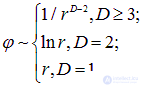
From expression (10.49) follows the behavior of the potential in an -dimensional world:
|
|
(10.50) |
These formulas are a consequence of the fact that differentiating the potential (the operation grad) must give the expression for the electric field strength.
This leads to curious conclusions. Since in one- and two-dimensional worlds the potentials grow without bound at infinity, an infinitely large amount of work is needed to separate two attracting charges. This means that in worlds of low dimensionality only finite motion of two attracting bodies (charges, masses) is possible. Recall that motion within a bounded region of space is called finite. Therefore, in worlds with  it is impossible to ionize an atom, impossible to launch a satellite beyond the Solar System, and so on. In such a world there would be no chemical reactions, and galaxies and stars could not evolve. In short, life there would be stagnantly dull.
One might expect a more pleasant existence in multidimensional  worlds. Alas, this too turns out to be an illusion. A study of the equation of motion
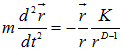
leads to the conclusion that at  finite motion essentially does not exist: it is realized only for circular orbits, and even then it is unstable — the slightest perturbation leads to the electron (planet) falling onto the attracting center or escaping to an infinitely large distance. It turns out that in such a world atoms, planetary systems, and everything else could not have formed at all. No stability whatsoever in worlds of higher dimensionality — that is the alternative to the «stagnant» low-dimensional worlds. Only at
  is both stable finite and infinite motion possible. It turns out that three-dimensional space is the only convenient form for the existence and motion of matter, at least of the kinds known to us that we study in physics.
Let us begin with the simple case where one of the two interacting systems is a single charge  . The charges of the other system will be denoted
  , where
  is the number of the charge in the system. Then the force of their interaction, namely: the force acting on the charge
  , according to the superposition principle, can be written in the form
|
|
(1.61) |
Here  and
and  — are the position vectors of the points at which the corresponding charges are located. The second relation is simply a statement of Newton's third law for this case. It must be emphasized that we are talking, throughout, about the force of interaction.
If two systems of charges, the first: 
 ,
,  and the second:
 ,
,  interact with each other, then the force of this interaction can be written in the form of the following double sum
|
|
(1.62) |
Here, as before,  and
and  — are the position vectors of the points at which the corresponding charges are located.
The formula, at least in principle, solves the problem of calculating the Coulomb (electrostatic) interaction forces of arbitrary systems of stationary point charges.
By a physically infinitesimal element is meant an element which, on the one hand, is so small that under the conditions of the given problem it can be considered a point mass, and, on the other hand, is so large that the discreteness of the charge (see relation) of this element can be neglected.
Let us make a necessary, in our view, additional clarification regarding the words «physically infinitesimal» volume. Such a volume should not be regarded as the result of a formal, purely mathematical limiting transition to zero. A physically infinitesimal volume is a volume whose size  , on the one hand, is small compared with any characteristic length in the problem under consideration
  (recall that in different problems these are lengths of quite different magnitude) and it can be considered a point. On the other hand, it is macroscopically large, that is, its size
  is large compared with the average distance between the particles
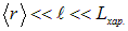
  (atoms, molecules, ions, electrons, etc.) making up the substance, so that the number of these particles inside the physically infinitesimal volume is macroscopically large. Correspondingly, the fact that this number changes discretely can be neglected. Thus, the linear size of a physically infinitesimal volume must satisfy the following inequality
Let us also note that quantities of the form  can of course be regarded as derivatives, but it is simplest, most convenient, and most productive to regard them as fractions: this is the ratio of the charge
  in the volume
  to the magnitude of this volume.
Two bodies  and
and  with volumes
  and
and  are charged with densities
  and
and  . In the first body, in the vicinity of a point with position vector
  , let us select a physically infinitesimal volume
  , inside which there is a charge
 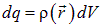 . Quite similarly, in the second body, in the vicinity of a point with position vector
  , let us select a physically infinitesimal volume
  , inside which there is a charge
 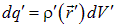 . Both volumes can be considered point charges; in accordance with Coulomb's law, let us write the expression for the force of their interaction:
|
|
(1.63) |
Note that the first relation differs from the corresponding one only in notation. In the latter expression the values of the charges  and
and  are simply substituted. Now, according to the superposition principle, it is necessary to sum over all pairs of point charges
  and
and  of which the first and second bodies consist. The difference is only that infinitesimal interaction forces of pairs of infinitesimal charges are summed, and there are infinitely many of them. The sum of an infinitely large number of infinitesimal quantities is an integral. Therefore, in the expression that is the result of such a summation, instead of the sums

we must write integrals over the volumes of both bodies  As a result we obtain
|
|
(1.64) |
The reader should be reassured: we will not have to calculate sixfold integrals here, any more than the threefold integrals describing the force of interaction of a single point charge and an extended body
|
|
(1.65) |
with a charge uniformly distributed over it with density  .
.
Let us consider examples of the application of these formulas.
Example 7. A conducting disk of radius  rotates with angular velocity
  Given that the current in the conductor is carried by electrons, determine the potential difference between the axis of the disk and its periphery.
Solution. Let us first obtain an estimate of the result using dimensional analysis. At our disposal are — the charge of the electron  and its mass
  , the angular velocity
  and the radius of the disk
  .
.
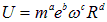
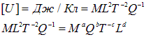
The desired formula must have the form:
|
|
|
Substituting the dimensions, we obtain:
|
|
|
from which follow the equations (which, in this case, are also the solution to the problem):
|
|
|
|
|
|
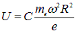
Let us now solve the problem exactly. In order for an electron located inside the disk at a distance  from the axis to move in a circle, a centripetal force must act on it:

This force is provided by a redistribution of the electron concentration in the disk, creating a radial electric field E. The equilibrium condition for the electron:
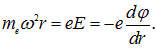
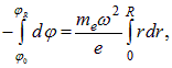
where  — is the potential at the center (at the periphery) of the disk.
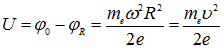
Here  is the linear velocity of points at the periphery of the disk. In principle, the formula obtained can be used to determine the ratio of the electron's charge to its mass. In practice, however, this is extremely difficult. Let us give an estimate. The charge of the electron is
  , its mass
 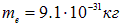 . Let us take the velocity at the periphery of the disk to be equal to 300 m/s. The potential difference arising between the axis and the periphery of the disk will then turn out to be equal to
  . Such a voltage is very difficult to measure in a moving system.
Example 8. A spherical drop of water, carrying an electric charge  has potential
  on its surface. What is the radius
  of the drop? What will be the value of the potential
  on the surface of the new spherical drop formed by the merging of two former ones? What is the dependence of the potential on the surface of the new drop, formed by the merging of several old ones, on their number n?
Solution. The potential on the surface of a charged sphere (or ball — in this case it gives the same result) is equal to

from which we find the radius of the drop:

When n drops of volumes  merge, a new drop is formed with radius
  and volume increased by a factor of
  :
:
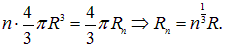
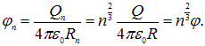
The new drop will also carry an increased charge:  From this we find for the potential on its surface:
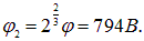
When two drops merge, we obtain for the potential
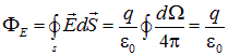
Let us consider the general derivation of Gauss's theorem. It is based on a direct calculation of the flux of the field-strength vector of a point charge through a closed surface  of arbitrary shape. As before, let us place the origin of coordinates at the point in space where, for now, the single charge
  is located (see Fig. 1.59).
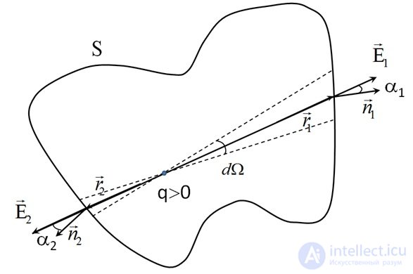
Fig. 1.59. Charge inside the surface
With the solid angle  let us «cut out» on opposite sides of the surface
  two small areas
  and
and  , with outward normals to the areas
  and
and  , and field strengths
 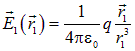 and
and 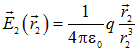 , respectively. The contributions to the flux from these two areas
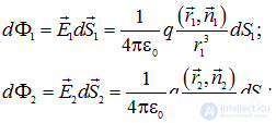
The scalar products entering the expressions for the fluxes are, evidently, equal to: 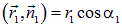 and
and 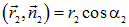 . Both areas under consideration do not lie on spherical surfaces, so their areas are larger by a factor of «|cos(α)|» than those of areas cut out by the same solid angle but on spherical surfaces of the corresponding radii (
  and
and  ), so the areas of the surface elements we are considering are equal to
  and
and 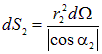 . In this case it is necessary to write precisely the absolute value of the cosine, since the area cannot be negative, while the angles can be obtuse and, correspondingly, the cosines — negative. Substituting the scalar products and the areas of the surface elements into the expressions for
  and
and  , we obtain
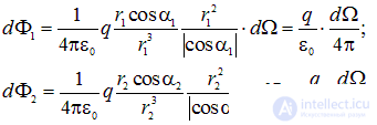
In the formulas written above it is taken into account that, in the case when the charge  is located inside the surface
  both angles (
  and
and  ) are acute, both cosines are positive, and in both cases
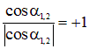
The expressions for  and
and  are identical, so for any surface element
  we can write
  ; integrating over the entire surface, as before, we obtain
|
|
(1.66) |
Let us note that the equality of the fluxes  and
and  is explained quite simply: 1) the areas of the surface elements grow with increasing distance to the point where the charge is located, proportionally to the square of this distance, while the magnitude of the field strength decreases inversely proportional to the square of the same distance; 2) by virtue of the central nature of the field of a point charge, the scalar product
  (in the numerator) and the ratio of the areas (in the denominator) both contain the cosine (in the first case) and the absolute value of the cosine (in the second case) of one and the same angle. Thus, the equality of the fluxes and is a consequence of the properties of the field of a point charge: its centrality and the law of decrease
  , that is, ultimately — Coulomb's law.
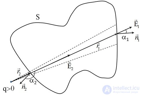
Fig. 1.60. Charge outside the surface
If the charge  is located outside the surface
  , then one of the two angles (see Fig. 1.60) is obtuse, and, for example, as in Fig. 1.59:
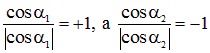 ,
,
then the sum
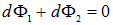 .
.
In this case, integrating over the entire surface, we have
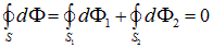
In the last expression,  — is the «far» part of the surface from the charge
  , on which
  , and
, and  — is the «near» part relative to the charge
  , on which
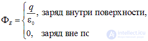
  . Combining both results, and for a surface of arbitrary shape, we obtain:
|
|
(1.67) |
The derivation of Gauss's theorem in general form can also be found, for example, in the textbook I.E. Tamm, «Fundamentals of the Theory of Electricity», Moscow, Nauka, 1989, p. 18.
Let us obtain a formula, very useful in practice, for calculating the gradient of a scalar function possessing spherical
|
|
(1.68) |
or cylindrical
|
|
продолжение следует...
Часть 1 1. The electric field in vacuum
Часть 2 1.4. Flux of a vector. The Ostrogradsky–Gauss theorem for a
Часть 3 1.5. Application of Gauss's theorem for calculating the electric field
Часть 4 Appendices - 1. The electric field in vacuum
Часть 5 - 1. The electric field in vacuum













Comments