
Lecture
Time and again, the ideas of quantum physics radically shattered established notions of how the world is built. We have already seen how, at a new level, particles that seemed long since discarded by science — photons, quanta of light — found their way into wave theory. In this chapter we will see how waves invaded and took the most honored place in that area of physics which had long since been firmly settled by particles. In a certain sense, quantum physics brought about an even more revolutionary upheaval in our knowledge than the theory of relativity.
Let us go back to the year 1911. By this time the discreteness of the microworld had shown up most vividly in atomic spectra. It turned out that atoms absorb and emit light only of a definite wavelength, with the spectral lines grouping into so-called series (Fig. 3.1).
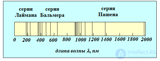
Fig. 3.1. Wavelengths radiated by the hydrogen atom: the spectrum consists of series (the first three are shown) —
sequences of lines converging toward a certain limiting minimum value (its own for each series)
 ; only four lines of the Balmer series lie in the visible range
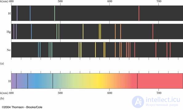
Fig. 3.2. (a) Line emission spectra of gaseous hydrogen, mercury, and helium: (b) absorption spectrum of hydrogen

Fig. 3.3. Continuous emission spectra are given by heated solids and liquids, strongly compressed gases, and high-temperature plasma
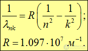
For the spectrum of hydrogen, the simplest of atoms, a simple formula was established (not derived, but guessed!)
|
|
|
(3.1) |
Here  — is the wavelength of radiation of the hydrogen atom, n and k > n — are integers, R — is the so-called Rydberg constant (
 , where
  — is the non-SI unit of energy «Rydberg», equal to half the atomic unit of energy). It turned out that the Lyman series is described by this formula for the values
  , the Balmer series — for
  , the Paschen series — for
  , and so on. The limiting (minimum) values for the wavelengths are obtained from (3.1) for
  :
:

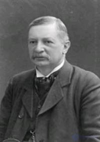
Fig. 3.4. Johannes Robert Rydberg (1854–1919)
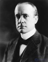
Fig. 3.5. Theodore Lyman (1874–1954)
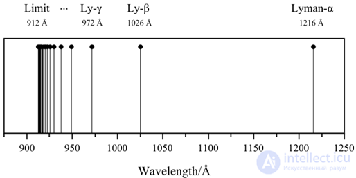
Fig. 3.6. The Lyman spectral series
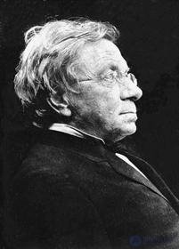
Fig. 3.7. Johann Jakob Balmer (1825–1898)

Fig. 3.8. Visible hydrogen emission lines in the Balmer series. Hα — the red line on the right, with a wavelength of 656.3 nm. The leftmost line — Hε, corresponds to radiation already in the ultraviolet region of the spectrum, at a wavelength of 397.0 nm
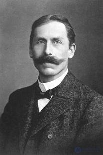
Fig. 3.9. Louis Carl Heinrich Friedrich Paschen (1865–1947)

Fig. 3.10. All lines of the Paschen series lie in the infrared range
Furthermore, as a result of studies of the properties of gases, it was known by that time that the sizes of atoms are approximately
equal to  . Therefore a theory explaining the spectrum and the sizes of atoms had to include some parameter allowing a quantity with the dimension of length to be constructed (the constants e and m — the charge and mass of the electron — are not sufficient for this). No such parameter existed in classical theory. The Rydberg constant could have been such a parameter, but its origin was obscure and mysterious.
In 1911, E. Rutherford published a theoretical paper (Rutherford E., Philosophical Magazine, v. 21, p. 669–688, 1911), in which, based on an analysis of experiments carried out in 1908–1909 by his students — the intern Hans Geiger and the graduate student Ernest Marsden — (Geiger H., Marsden T., Proceedings of the Royal Society of London, Series A, v. 82, p. 495–499, 1909) he asserted the existence, inside the atom, of a positively charged nucleus, in which practically the entire mass of the atom is concentrated.
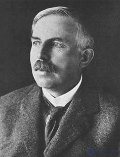
Fig. 3.11. Ernest Rutherford (1871–1937)
Later, in one of his lectures, E. Rutherford himself recalled those times as follows (quoted from the book by G. Trigg, Landmark Experiments in Twentieth Century Physics, Moscow, «Mir», 1974, p. 77): «…I remember… Geiger came to me, greatly excited, and said: «We have got some of the  — particles coming back…». It was quite the most incredible event that has ever happened to me in my life. It was almost as incredible as if you fired a 15-inch shell at a piece of tissue paper and it came back and hit you. On consideration, I realized that this scattering backwards must be the result of a single collision, and when I made calculations I saw that it was impossible to get anything of that order of magnitude unless you took a system in which the greater part of the mass of the atom was concentrated in a minute nucleus. It was then that I had the idea of an atom with a minute massive centre, carrying a charge». We should add that the words «scattering backwards» actually meant scattering through 150 degrees, since the design of the apparatus used at that time did not allow scattering at larger angles to be observed.
The basic scheme of Rutherford's experiments is shown in Fig. 3.12. A diagram of the actual apparatus can be found in the above-cited book by G. Trigg.
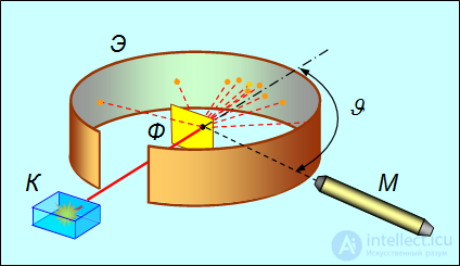
Fig. 3.12. Diagram of Rutherford's scattering experiment on  — particles
From a radioactive source enclosed in a lead container,  particles were directed onto a thin foil F of the metal under study. The scattered particles struck a screen coated with a layer of zinc sulfide crystals, capable of glowing under the impact of fast charged particles. Scintillations (flashes) on the screen were observed by eye with the aid of a microscope. Observations of the scattered particles in Rutherford's experiment could be carried out at various angles
  to the original direction of the beam. It was found that most particles pass through the thin layer of metal, practically without experiencing deflection. However, a small fraction of the particles are deflected through significant angles, exceeding 30°. Very rare particles (approximately one in ten thousand) were deflected through angles close to
  . It is clear that an particle can be thrown backward only if the positive charge of the atom and its mass are concentrated in a very small volume within the atom. In this way the atomic nucleus was discovered — a body of dimensions small in comparison with the atom, in which the entire positive charge and practically the entire mass of the atom are concentrated. The size of the nucleus was estimated by E. Rutherford in his 1911 paper; the estimate gave a value less than or of the order of
  .
.
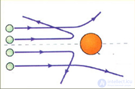
Fig. 3.13. Diagram of the scattering of alpha particles on the nucleus of a gold atom
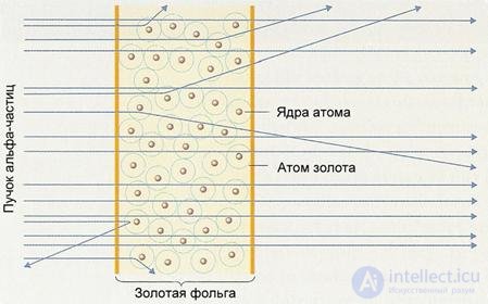
Fig. 3.14. Diagram of the scattering of a flux of alpha particles in a thin gold foil
A planetary model of the hydrogen atom arose: a proton with an electron in orbit. Physicists love unified models, and here, so elegantly, the small repeated the large — in the atom, the Solar System.
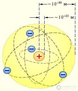
Fig. 3.15. Diagram of Rutherford's nuclear (planetary) model of the atom
The problem was that an electron undergoing finite, and therefore accelerated, motion around the nucleus must fall onto the nucleus. The point is that the electron is charged, and during accelerated motion it must emit electromagnetic radiation, that is, stationary motion is impossible. Classical electrodynamics predicts that, having rapidly lost its energy and the angular momentum of its orbital motion, the electron must fall onto the nucleus in about  . In this time, light travels about 1.5 cm (it would seem that we see only «dead» atoms, but this is not so!). Rutherford understood the problem, but deliberately concentrated on the fact of the nucleus's existence, believing that the question of the stability of the atom would be resolved through investigation of the behavior of atomic electrons. This was destined to be done in 1913 by N. Bohr, who proposed a new theory of the atom.
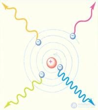
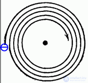
Fig. 3.16. Instability of the Rutherford model of the atom
Bohr's postulates
Bohr's first postulate
|
In an atom there exist stationary orbits, on which the electron does not radiate. |
Here we can trace the «forcible» introduction of discreteness (not all orbits are allowed), as well as something typical of physics — «sweeping the problem under the rug»: if no explanation can be found for something, it is accepted as a given and its consequences are studied in the hope that the cause will someday be understood.
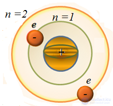
Fig. 3.17. Illustration of Bohr's first postulate
Bohr's second postulate
|
When passing from one stationary orbit to another, the electron emits (absorbs) a quantum of light with frequency
( |
This postulate reflects conservation of energy and the Planck – Einstein relation.
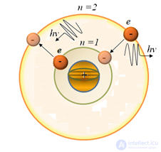
Fig. 3.18. Illustration of Bohr's second postulate
Bohr's third postulate
|
The dynamics of the electron on a stationary orbit is determined by the equations of classical theory. |
An inevitable consequence: since the remaining orbits are forbidden for the electron, the transition occurs as a jump; it makes no sense to speak of the electron's path or energy between orbits — the laws of mechanics do not apply there.
Bohr's fourth postulate
|
Circular stationary orbits are determined by the condition of quantization of angular momentum (n — an integer):
|
Planck's constant ħ has the dimension of angular momentum and, together with the electron charge e and its mass m , makes it possible to form a parameter of the dimension of length. This makes it possible to calculate the size of the atom.
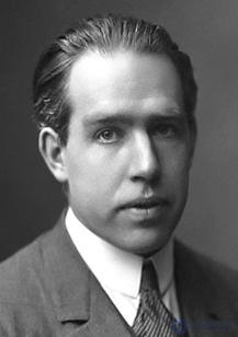
Fig. 3.19. Niels Henrik David Bohr (1885–1962)
Application of Bohr's postulates
Classical mechanics for an electron revolving in a circular orbit of radius R with speed v around a nucleus of charge Ze, gives the equation of motion
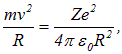
whence
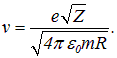
Therefore the energy E and angular momentum L of the electron are expressed in terms of the orbit radius R:
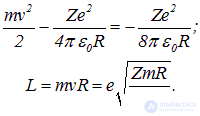
If Bohr's quantization condition L=nħ (n=1, 2, 3, …) is applied to the last expression, the following results are obtained.
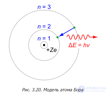
Fig. 3.20. The Bohr model of the atom
Characteristics of the hydrogen-like atom
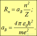
Radii of the allowed orbits
|
|
|
(3.2) |
Energy of the electron on a stationary orbit
|
|
|
(3.3) |
The constant aB , which has the dimension of length, is called the Bohr radius:  . The meaning of the number
  — is the number of the allowed orbit. The Bohr radius — is the radius of the lowest orbit
  in the hydrogen atom
  .
.
Formula (3.3) determines the discrete values of energy that the electron can have in the hydrogen atom, or, as they say, the energy levels. Negative values of  correspond to bound states of the electron in the atom, that is, to motion in a limited region of space (the analog in classical physics — the motion of planets along ellipses, as opposed to hyperbolic and parabolic trajectories that go off to infinity).
When solving problems about the behavior of an electron in an atom, expressions usually arise that include the square of the electron's electric charge in combination with the electric constant
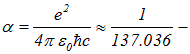
  . It is quite useful to introduce a dimensionless combination of fundamental world constants — the so-called fine-structure constant:
|
|
|
(3.4) |
which, together with the atomic number  and the orbit number
  , determines the scale of relativistic effects in the atom. To make this more visible, let us rewrite formula (3.3) so that the fine-structure constant enters its right-hand side:

Because of the factor  , the energies characteristic of an atom turn out to be four orders of magnitude smaller than the electron's rest energy. This is a manifestation of the non-relativistic nature of sufficiently light
  atomic systems. As can be seen from the last expression in the formula above, relativistic effects cease to be small corrections for electrons close to the nucleus
  in heavy
  atoms.
Example 1. Let us determine the speed of the electron on the nth orbit of the Bohr atom. The radius of the nth orbit is determined by the formula

where aB — is the Bohr radius. The electron speed v can be expressed in terms of the angular momentum L=nħ:
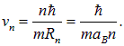
The expression for the Bohr radius may be simplified using the introduced fine-structure constant:
|
|
|
(3.5) |
Substituting this expression into the formula obtained above for the electron speed, we get for the nth orbit

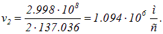
From this it follows that on the lowest orbit the electron's speed is approximately 137 times less than the speed of light, that is, the atom is indeed a non-relativistic system. On the nth orbit the electron's speed is n times less than on the first. Numerical example: on the second orbit the electron's speed equals
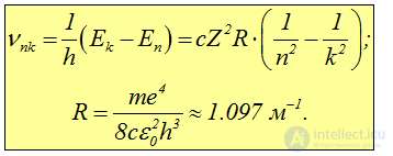
When transitioning from level k to level  the excess energy
  goes over into the energy of a photon
  . Therefore for the spectrum of emitted frequencies we obtain the relation (cf. (3.1))
|
|
|
(3.6) |
Thus, Bohr's theory also made it possible to calculate the Rydberg constant . The existence of spectral series, and of the limiting values
  (Fig. 3.21), also became understandable.
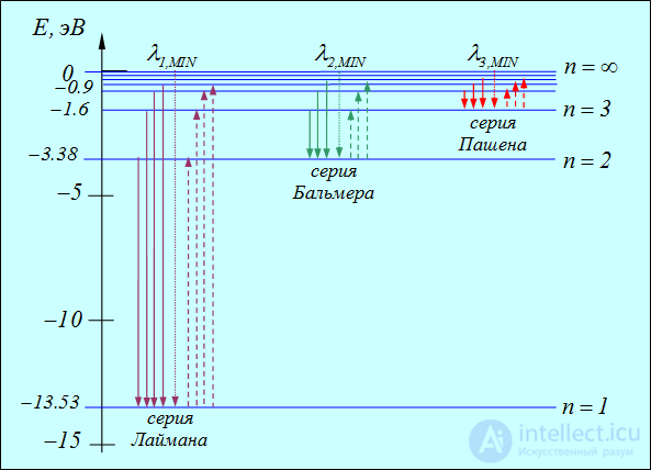
Fig. 3.21. Diagram of the energy levels and transitions in the hydrogen atom according to Bohr's theory:
solid lines (top-to-bottom transitions) — emission, dashed lines (bottom-to-top transitions) — absorption.
The boundaries (limits) of the series  are shown, to which correspond transitions from a level with
 — boundaries between the continuum and the discrete spectrum
Experimental confirmation of Bohr's assertion about the discreteness of the energy spectrum of atoms was found in the Franck–Hertz experiments, which consisted in bombarding mercury vapor with electrons in a vacuum tube and measuring the dependence of the anode current on the accelerating potential difference. A diagram of the experiment is shown in Fig. 3.22.
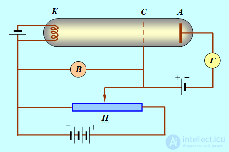
Fig. 3.22. Diagram of the Franck – Hertz experiment
The tube, filled with mercury vapor at low pressure (about 1 mm Hg), contains three electrodes: an anode, a cathode, and a grid. Electrons leaving the surface of the heated cathode owing to thermionic emission are accelerated by the voltage U, applied between the cathode and the grid. This voltage can be varied using a potentiometer P. Between the anode and the grid a weak retarding field is applied, with a potential difference of about 0.5 V, which slows the motion of electrons toward the anode. The dependence of the current I in the anode circuit on the applied voltage U was determined. The results obtained are shown in Fig. 3.23.
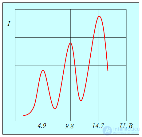
Fig. 3.23. Dependence of the current I in the anode circuit on the applied voltage U in the Franck — Hertz experiment
The current initially increases monotonically, reaches a maximum at a voltage of 4.9 V, after which, as U increases, it drops sharply, reaches a minimum, and starts to rise again. The current maxima recur at voltages of 9.8 V, 14.7 V, and so on. The alternation of maxima at equal distances from one another proved the discreteness of the change in the atom's energy.
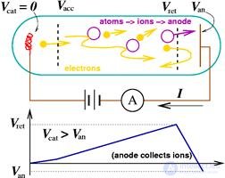
Fig. 3.24. Inelastic collisions of electrons with mercury atoms
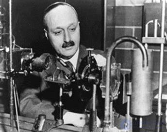
Fig. 3.25. James Franck (1882–1964)
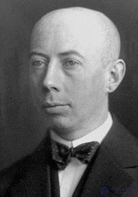
Fig. 3.26. Gustav Ludwig Hertz (1887–1975)
Example 2. When transitioning from the third level to the second (the head line of the Balmer series), a hydrogen-like ion of a certain element emits a photon with an energy of 7.5 eV. Let us determine which element this is.
The energy of an electron located on the nth orbit around a nucleus of charge Ze, equals
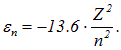
When transitioning from level n  to level
  the energy released is

whence
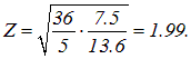
The atomic number of an element is an integer, so after rounding we obtain Z = 2, which corresponds to helium.
As noted above, even before the appearance of Bohr's theory the spectrum of the hydrogen atom had been studied and formula (3.1) established empirically. But when observing the solar spectrum, lines were noticed that seemed to violate this formula, since they corresponded to half-integer values of n and k. After the appearance of Bohr's theory it became clear that the quantum numbers n and k must nevertheless be integers, and that the apparent half-integer values could be explained differently. Indeed, from formula (3.6) for the frequencies emitted by a hydrogen-like atom, it follows that
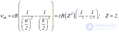
that is, the observed lines belong to an ion of the element with Z = 2. As is known, this element bears the «solar» name — helium.
So again, discreteness, mysterious integers. In classical physics they appeared in interference phenomena (the numbers of maxima and minima) and in standing waves (the number of nodes on strings). In 1923 a fundamental hypothesis of Louis de Broglie was put forward:
|
Wave–particle duality of photons is inherent in all microparticles. |

Fig. 3.27. Louis Victor Pierre Raymond, 7th Duke de Broglie, better known as Louis de Broglie (1892–1987)
We were forced to attribute a momentum to the photon

For a long time attention was paid only to its wave properties, and in the 20th century its corpuscular properties were also restored to good standing. With the electron the opposite happened: it was de Broglie alone who discerned oscillations in it with a wavelength  . Bohr's quantization condition

received a simple interpretation. It became the condition that an integer number of wavelengths fit along the length of the stationary orbit:

(an analogy with wallpaper: if an integer number of pattern periods fits around the perimeter of a room, then when the papering continues the pattern is reproduced at the same places — a kind of stationarity). From this the relation follows

It can be seen that we have obtained a general formula for photons and electrons (and any other particles).
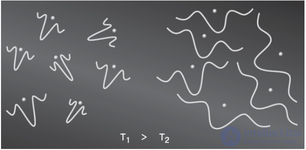
Fig. 3.28. Every particle (atom, molecule) can be represented as a de Broglie wave or a wave packet, whose center corresponds to the center of the particle. As it cools, that is, as the speed of the particle's random motion decreases, the wavelength grows, and the wave packets of particles eventually overlap. (Image: «Chemistry and Life»)
De Broglie's hypothesis was confirmed by the experiments of Davisson and Germer (reflection from crystal planes) and of Thomson (diffraction on a foil). The experiment of V.A. Fabrikant (1949) — diffraction of single electrons — is beautiful and instructive, proving that wave properties belong not to a collective of particles but to each electron individually. And at the same time the electron is a particle with charge and mass.
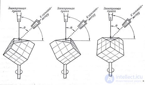
Fig. 3.29. Diagram of the Davisson and Germer electron diffraction experiment (C. J. Davisson, The discovery of electron waves, Les Prix Nobel en 1937.) A beam of electrons of a definite speed is directed onto the plane of a nickel crystal, shown as a cube with a cut-off corner. The Faraday cylinder, used to collect the diffracted electrons, can move along an arc around the crystal. The figure shows three different positions of the crystal
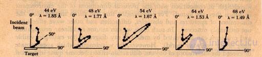
Fig. 3.30. The Davisson and Germer electron diffraction experiment. Polar diagrams of the intensity of elastically scattered electrons for different energies of the primary beam
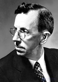
Fig. 3.31. Clinton Joseph Davisson (1881–1958)
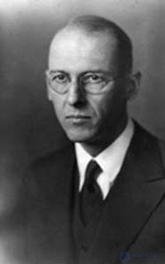
Fig. 3.32. Lester Halbert Germer (1896–1971)
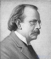
Fig. 3.33. Sir Joseph John Thomson (1856–1940)
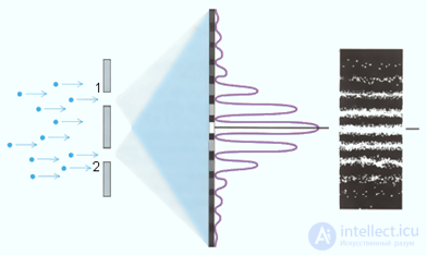
Fig. 3.34. Diagram of electron diffraction through two slits
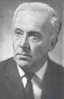
Fig. 3.35. Valentin Alexandrovich Fabrikant (1907–1991)
A question that long troubled physicists: what is a microparticle, a wave or a corpuscle? Here we have an incorrectly posed question, implying an alternative. We must replace «or» with «and»: the electron is both a wave and a particle. If we pose this question to nature with the help of an instrument, we get an answer corresponding to the instrument: for a wave instrument (for example, a diffraction grating) the answer will be «wave», for a corpuscular one (say, a counter) — «particle». The ambiguity of the answer reflects the duality of the nature of particles, or, more precisely, the narrowness of our alternative-based thinking, which allows for only one of these possibilities. These are new objects for us, the quantum mermaids and centaurs of the microworld, which cannot be divided into people and animals. In this sense a microobject is neither a wave, nor a particle, nor their symbiosis. It is a new quality, which we express quantitatively in the de Broglie formula
|
|
|
(3.7) |
linking the wave and corpuscular manifestations of the properties of a single object. In experiments with accelerated particles, their de Broglie wavelength plays the same role as the wavelength of visible light does in determining the resolving power of a microscope. Accelerators are a kind of microscope of the microworld, and they are used to study the laws of nature at small distances. Thus, the wavelength of protons obtained at the accelerator in Serpukhov is about 10 –17 mm, which is 10 7 times smaller than the size of atoms.
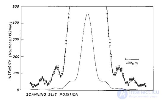
Fig. 3.36. An experiment with neutron diffraction through a slit 90 µm wide. The de Broglie wavelength for the neutron beam is λ = 1.926 ± 0.07 ± 0.002 nm (mean wavelength, spread in the beam, measurement error). The experiment took about 320 hours, with measurements carried out over two weeks at a nuclear reactor with a high neutron flux. The graph shows the general form of the dependence, as well as the same graph at an enlarged scale, in order to better show the higher-order diffraction maxima. The experimental points are plotted with their errors indicated, and the solid curve is the result of the theoretical calculation. The positions of the maxima and their amplitude both agree with the experiment. (Zeilinger et al. Rev. Mod. Phys., 1988, 60, 1067–1073)
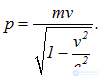
When solving problems related to the de Broglie wavelength, formula (3.7) must be applied with care. It is necessary to understand clearly which expression for the momentum should be used. For example, a problem may specify the particle's speed v. If this speed is much less than the speed of light in vacuum, the classical relation may be applied

In practice, it is considered that v<<c, if the ratio v/c<0.3, that is

If this is not the case, then the relativistic relation between the momentum of the particle and its speed must be used
A problem may specify not the particle's speed but its kinetic energy K. The criterion for the applicability of the classical formulas is that the kinetic energy be small compared with the particle's rest energy  . If the condition

is satisfied (which, as is easy to see, is equivalent to the condition  ), then the momentum can be found using the formulas of classical mechanics
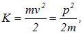
whence

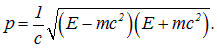
If the kinetic energy of the particle is not small compared with the rest energy (and especially if it exceeds it), then relativistic formulas must be used. Relativity theory derives a general relation between the total energy of a particle and its momentum:
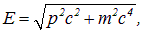
whence
|
|
|
(3.8) |
The kinetic energy equals the difference between the total energy and the rest energy:

so that for the momentum we obtain
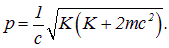
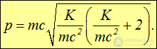
Finally, it is convenient to rewrite this expression so that dimensionless quantities stand under the square root sign:
|
|
|
(3.9) |
It is easy to verify that when

formula (3.9) indeed passes over into the classical expression

Traditional units of energy (for example, J) turn out to be inconvenient in the microworld. Physicists therefore prefer to use the non-system units already familiar to us — the electron-volt (eV) and its derivatives (1 keV = 103 eV, 1 MeV = 106 eV , 1 GeV = 109 eV and so on).
|
The electron-volt (1 eV) is the energy acquired by an electron on passing through a potential difference of 1 V. |
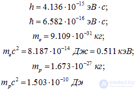
Since the electron's charge equals e = 1.602·10–19C , then 1 eV = 1.602·10–19 J. Now that the concept of rest energy has appeared, let us give its numerical values for the electron and the proton together with the masses of these particles. Let us also give the numerical value of Planck's constant expressed in eV·s:
|
|
|
(3.10) |
Finally, there are inverse problems, in which the de Broglie wavelength l is given and one must find the speed or energy of the particle. The question arises of how, from the value  alone, to determine which formulas should be used. Let us suppose that we apply the classical formula to find the speed

and consequently obtain

The criterion for the validity of this result is that v be small compared with the speed of light in vacuum c:

whence

The combination of constants

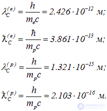
is the particle's Compton wavelength. Physically, this is the characteristic distance defining the region  , where non-relativistic quantum mechanics is no longer applicable. Let us give the numerical values of this important parameter for the electron and the proton:
|
|
|
(3.11) |
It can be seen that the lighter the particle, the larger its Compton wavelength, that is, the sooner relativistic effects appear. For the electron, the Compton wavelength is much smaller than the characteristic length that determines the size of an atom. This means that non-relativistic quantum mechanics applies to the atom. Nuclei, composed of protons and neutrons, have sizes on the order of 10–14 mm, which is much larger than the proton's Compton wavelength. Consequently, this theory applies to them as well.
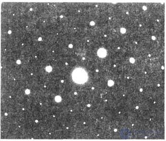
Fig. 3.37. Diffraction pattern obtained when a beam of electrons (E = 75 kV, λ = 0.05 Å) passes through a single-crystal ZnSe film with (111) orientation
Example. Let us determine the speed of a particle whose de Broglie wavelength is 10 times smaller than its Compton wavelength  .
.
By the condition

whence we find

Since the de Broglie wavelength is smaller than the particle's Compton wavelength, we cannot use the non-relativistic relation

which would lead to the absurd answer v=10c (as is known, nothing can move faster than light). Here it is necessary to apply the relativistic formula relating momentum to speed
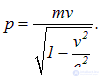
From this the equation follows
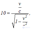
whose solution gives
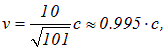
that is, the particle's speed is only 0.5 % less than the speed of light.
The mere presence of wave properties in a particle imposes certain restrictions on the possibility of a corpuscular description of its behavior. For a classical particle it is always possible to specify its exact position and momentum. For a quantum object we have a different situation.
Let us imagine a wave train of spatial extent  — the image of a localized electron, whose position is known to within
  . The de Broglie wavelength for the electron can be determined by counting the number N of spatial periods on the segment :

What is the accuracy of determining  ? It is clear that for a slightly different wavelength we would get approximately the same value of N. An uncertainty
  in the wavelength leads to an uncertainty
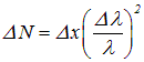
in the number of nodes, and only  are accessible to measurement. Since

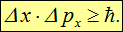
it immediately follows that this is the famous V. Heisenberg uncertainty relation for coordinates — momenta (1927):

For the sake of precision it should be noted that, firstly, the quantity  in this case means the uncertainty of the projection of the momentum onto the axis OX and, secondly, the reasoning given is more qualitative than quantitative in character, since we have not given a rigorous mathematical formulation of what is meant by the uncertainty of a measurement. Usually the uncertainty relation for coordinates-momenta is written in the form
|
|
|
(3.12)
|
Analogous relations hold for the projections of the position vector and momentum of a particle onto the two other coordinate axes:
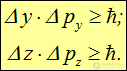
Let us now imagine that we stand still while an electron wave passes by. Observing it for a time  , we want to find its frequency n. Having counted
  oscillations, we determine the frequency with accuracy
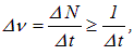
whence we have

or (taking into account the relation  )
)

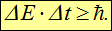
Analogous to inequality (3.12), the Heisenberg uncertainty relation for the energy of a system is more often used in the form
|
|
|
(3.13) |
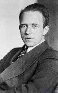
Fig. 3.38. Werner Karl Heisenberg (1901–1976)
Let us discuss the physical meaning of these relations. One might get the impression that they reflect an «imperfection» of macroscopic instruments. But the instruments are not at all to blame: the restrictions are fundamental in nature, not technical. The microobject itself cannot be in a state in which a definite value of one of its coordinates and of the momentum projection on that same axis are simultaneously possessed.
The meaning of the second relation: if a microobject lives for a finite time, then its energy does not have an exact value — it is, as it were, smeared out. The natural width of spectral lines is a direct consequence of Heisenberg's formulas. On a stationary orbit the electron lives indefinitely long, and its energy is determined exactly. This is the physical meaning of the concept of a stationary state. If the uncertainty in the electron's energy exceeds the difference between the energies of neighboring states

then it cannot be said exactly at which level the electron is. In other words, for a short time of order

the electron can jump from level 1 to level 2, without emitting a photon, and then return back. This is a virtual process, which is not observed and therefore does not violate the law of conservation of energy.
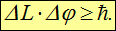
Similar relations exist for other pairs of so-called canonically conjugate dynamical variables. Thus, when a particle rotates around some axis in an orbit of radius R the uncertainty of its angular coordinate  entails an uncertainty in its position on the orbit
  . From relations (3.12) it follows that the uncertainty of the particle's momentum satisfies the inequality

Taking into account the relation between the electron's angular momentum L and its momentum L = Rp, we obtain  , whence follows one more uncertainty relation
|
|
|
(3.14) |
Some consequences of the uncertainty relations
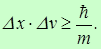
For massive objects the right-hand side is vanishingly small, which makes it possible to simultaneously measure the speed and position of an object (the region of validity of classical mechanics). In the Bohr atom, however, the electron's momentum
and the uncertainty of position turns out to be of the order of the orbit radius.
|
For example, for an oscillator (a mass on a spring) the energy E can be written in the form
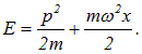
The ground state in classical mechanics is a state of rest at the equilibrium position:

Therefore the magnitude of the uncertainties  and
and  is of the order of the values of the momentum and coordinate themselves, whence we obtain
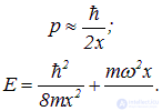
The minimum energy is reached at the point

and equals

Generally speaking, such estimates cannot claim to give an exact answer, although in this case (as for the hydrogen atom) it is indeed exact. We have obtained the so-called zero-point oscillations: a quantum oscillator, unlike a classical one, cannot remain at rest — this would contradict the Heisenberg uncertainty relation. Precise calculations show that Planck's formula for the energy levels of the oscillator should actually be written in the form
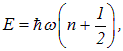
where n = 0, 1, 2, 3, ... is the vibrational quantum number.
When solving problems on the application of the uncertainty relation, one should keep in mind that in the ground state in classical physics the electron is at rest at the point corresponding to the minimum of the potential energy. The uncertainty relations do not allow it to do this in quantum theory, so the electron must have some spread of momenta. Therefore the uncertainty of the momentum (its deviation from the classical value 0) and the momentum itself coincide in order of magnitude

The uncertainty of the coordinate of an electron «locked» in a volume V, is, in order of magnitude, equal to the linear size of this volume

Example 1. An electron with kinetic energy  is located in a metallic dust particle of diameter
  . Let us estimate the relative inaccuracy dv, with which the electron's speed can be determined.
By the condition

and

The electron's energy is much less than its rest energy, so non-relativistic relations may be applied
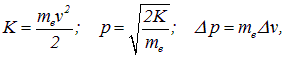
whence

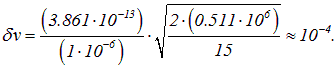
For the relative uncertainty of the electron's speed we obtain

In this expression the dimensionless factors are singled out — the ratio of the electron's Compton wavelength

to the diameter of the dust particle, and the ratio of the electron's rest energy to its kinetic energy. Substituting the numerical values:
Example 2. The average lifetime of an atom in an excited state is  . On transitioning to the ground state, a photon is emitted with wavelength
  (green color). Let us determine the energy of the quantum, and the width and relative width of the spectral line.
The energy of the quantum equals

The uncertainty in the energy is determined by the relation

whence

Then

Strictly speaking, we have not yet even become acquainted with quantum mechanics, but have only approached its threshold. Nevertheless, we can already give an estimate of the region in which the relations we have derived will certainly not be valid. If we approach the microworld from the side of the region of applicability of classical physics, no problems arise. Indeed, quantum relations do not cancel the classical laws at all, but refine them. In the macroworld, characterized by large values of energies and angular momenta, quantum discreteness is simply imperceptible, so that, generally speaking, both quantum and classical laws can be applied to macroscopic objects. The difference between the quantitative results obtained with their help will be negligibly small, but the classical laws are simpler. In this sense we speak of the region where the laws of classical physics are valid.
It is a different matter when we begin to advance deeper into the microworld. In principle it is clear that somewhere even the laws of quantum mechanics may fail, and scientists will have to devise some new theory. In this course we shall be dealing with non-relativistic quantum mechanics, which studies microobjects moving at speeds much less than the speed of light. We shall also encounter relativistic objects (photons and others), but we will note such cases specially.
Let us now determine the region of validity of non-relativistic quantum mechanics. Let us imagine a microparticle of mass m. The quantum uncertainty  of its energy must be much less than the rest energy
sup (otherwise the quantum effects would necessarily be relativistic, which would require a generalization of the theory). From the uncertainty relation (3.13) and the condition of applicability of the non-relativistic equations  follows a restriction on the time intervals:

The characteristic time

is thus the watershed between relativistic and non-relativistic quantum theories. In this time a particle can travel a distance no greater than
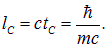
The quantity lC — is the characteristic distance at which the boundary between the non-relativistic and relativistic theories lies. For the electron it equals  and for the proton —
  The corresponding time intervals equal
  for the electron and
  for the proton.
In Fig. 3.6 distances are plotted on a logarithmic scale along the x axis, and speeds along the y — axis.
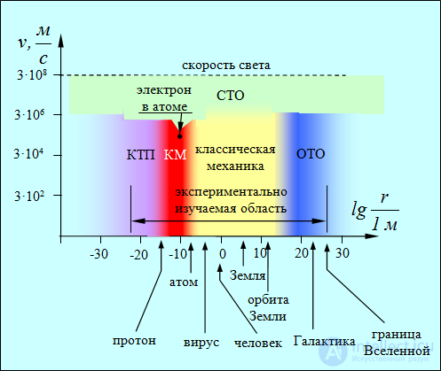
Fig. 3.39. Distance — speed diagram for a visual illustration of the regions of applicability of physical theories:
classical mechanics, special relativity (SR), quantum mechanics (QM),
general relativity (GR), and quantum field theory (QFT).
The point shows an electron in an atom — in the domain of quantum mechanics
The regions of applicability of the main physical theories are marked (GR — general relativity, SR — special relativity, QM — quantum mechanics, QFT — quantum field theory, also known as — relativistic quantum theory, also known as — the theory of elementary particles). The boundaries between the various theories are blurred, since they do not contradict one another but develop and complement each other. Thus, QFT, which deals with the properties of elementary particles, arose from the union of QM and SR, while GR (also known as the theory of gravitation) — arose from extending SR and classical mechanics to the region of large distances. The right-hand boundary of the QM region does not mean that quantum mechanics cannot be applied where we are accustomed to using classical mechanics. It is simply impractical to do so. Note that the figure is bounded on both sides. The Big Bang, in which our Universe was born, occurred, according to the current estimate, 14 billion years ago. In this time light has covered a distance of about 1026 mm, which determines the maximum possible distances in this world. At distances of about 10–35 m it is necessary to take gravitational forces into account, and no quantum theory of these has yet been created. Only very bold theorists venture to seriously discuss what happens at such small distances. Therefore this region is not shown in the figure.
Let us sum up this chapter. We have arrived at a contradictory picture of the microworld. In the Bohr atom, laws of motion along a classical trajectory were used, which turned out in the end to be incorrect. The calculation of the orbit radius and the electron's momentum contradicts de Broglie's wave ideas, from which we derived these very characteristics. Finally, it remains altogether unclear just what it is that oscillates in space as the electron moves.

 — the difference of the electron's energies on the orbits).





Comments