
Lecture
Even in ancient times it was known that certain minerals, such as magnetite (chemical composition
31% — Fe, 69% — O), are able to attract one another, and also attract pieces of iron. Such bodies are called magnets. The greatest attractive force is found at the opposite ends of a magnet, which are called magnetic poles.
The knowledge of the ancient world about magnets was minimal. Magnets found practical application in the Middle Ages, when an exceptionally important instrument — the compass — appeared. Its inventor is unknown. It was once believed that the compass, invented long ago in China, was brought to Europe by Marco Polo (1254–1324). However, there are written European sources from the 12th century that already describe the use of the compass, with its invention attributed to the Arabs. Some Chinese sources from about the same period attribute the invention of the compass to unknown foreign seafarers. Be that as it may, a magnetic needle placed on a pivot and free to rotate about a vertical axis made it possible to make many geographical discoveries.
At every point on the Earth's surface (in the absence of interference), a compass needle assumes a strictly defined direction: one end points approximately toward geophysical north, and the other — toward the south. The end of the compass needle that points north is conventionally called the north end (N), and the opposite end the south end (S) (Fig. 5.1).
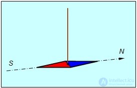
Fig. 5.1. Behavior of a compass needle in the Earth's magnetic field
If, in some region of space, forces act on a compass needle tending to set it in a definite direction, we say that a magnetic field exists there. The behavior of a compass needle in a magnetic field (of the Earth or of any other source) allows us to introduce magnetic induction lines (magnetic field lines) by analogy with the field lines of an electric field. In some sense this is even easier: the needle itself indicates the direction of the field line at the point where it is located. The main force characteristic of a magnetic field is the magnetic flux density vector B, directed tangent to the field line passing through a given point. At different points of the field, the induction has different values in magnitude and direction.
Figure 5.2 shows the orientation of a compass needle, which can rotate about horizontal and vertical axes, along the induction vector of the Earth's magnetic field, inclined at a certain angle to the horizon.
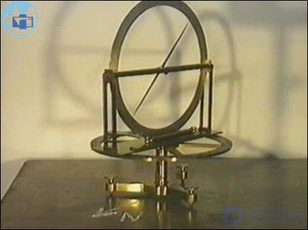
Fig. 5.2. Orientation of a compass needle in the Earth's magnetic field
Figure 5.3 shows that a current-carrying coil in the Earth's magnetic field behaves similarly to a compass needle. The axis of a long current-carrying coil, suspended on a thin thread in a horizontal position, orients itself along the horizontal component of the Earth's magnetic flux density vector, that is, in the north-south direction, just like an ordinary compass needle.
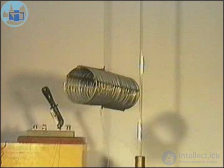
Fig. 5.3. Orientation of a long current-carrying coil in the Earth's magnetic field
Magnetic induction lines, unlike electrostatic field lines, are always closed. Speaking of the magnetic field of permanent magnets, it is customary to say that the lines emerge from the north pole of the magnet, enter the south pole, and close up inside the magnet (Fig. 5.4)
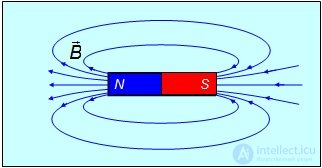
Fig. 5.4. Field lines of a permanent magnet
It has been established experimentally that unlike poles attract and like poles repel. In this sense, the interaction of magnets resembles the interaction of charged bodies. The behavior of a compass needle means that terrestrial magnetism exists, just as the Earth's gravitational field exists owing to its mass. Since the end of the needle facing north was called the north pole, and unlike poles attract, a south magnetic pole is located near the Earth's north geographic pole. In other words, the Earth's magnetic field is directed from south to north (Fig. 5.5).
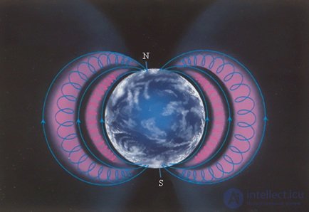
Fig. 5.5. The Earth's magnetic field: the north magnetic pole N is located near the south geographic pole.
The Earth's radiation belts are shown — the inner (proton) and outer (electron) belts —
where charged particles of cosmic rays are trapped by the magnetic field
The electrostatic field E is produced by electric charges and acts upon them, which we can symbolically depict as

The two poles of a magnet suggest a symmetric relation

It turns out, however, that the symmetry between magnetic and electric phenomena is not so straightforward. Whereas individual bodies can be charged either only positively or only negatively, since there exist elementary charged particles — carriers of electric charges of different signs — it is impossible to separate one magnetic pole from the opposite one. If a magnet is cut into two parts, each part again behaves as an independent magnet with opposite poles at its ends (Fig. 5.6).
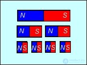
Fig. 5.6. When attempting to divide a magnet into two opposite magnetic charges (monopoles),
it turns out that each part still has two poles
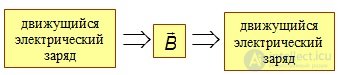
What would happen if, in dividing, we went so far as to break the magnet into individual atoms? Could the north pole then be separated from the south pole? No — even individual atoms behave as microscopic but nevertheless «full-fledged» magnets with north and south poles. It turns out that even individual elementary particles (for example, electrons) are micromagnets. At present there is no experimental evidence that separate magnetic charges (monopoles), analogous to electric charges, can exist in nature. It turns out that a magnetic field is produced by moving electric charges and, in turn, acts upon them, so that our scheme takes the form
|
|
(5.1) |
In everyday life we usually deal with small electric charges. At the same time, the charge flowing through the cross-section of a conductor, even at a modest current, is large owing to the enormous concentration of electrons in a metal. It is therefore not surprising that the first experimental observations of the connection between electric and magnetic phenomena followed the scheme
|
|
(5.2) |
If we understand the arrows in (5.2) as experimental confirmation of the indicated relation, then the first of them (the generation of a magnetic field by a current) was demonstrated by the Danish scientist H. C. Ørsted.
In 1820, Ørsted established experimentally that conductors carrying currents also interact with a compass needle. The scheme of Ørsted's experiment is shown in Fig. 5.7. Near a stationary wire laid along a meridian, a compass needle is placed, which, with the current switched off, lies parallel to the wire. When the current is switched on, the compass needle turns, tending to align itself perpendicular to the wire.
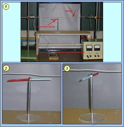
Fig. 5.7. Ørsted's experiment:
1 — scheme of the experiment; 2 — position of the needle with the current switched off; 3 — position of the needle with the current switched on
The position of a compass needle placed near a current-carrying conductor changes with a change in the direction of the current, but the needle does not react at all to stationary electric charges. From this we can conclude that only moving electric charges (electric current) are capable of creating a magnetic field, while around stationary charges there exists only an electrostatic field. The magnetic field arising in the space around current-carrying conductors, like the electric field due to stationary charges, is a form of matter. As we shall soon see, it possesses definite physical properties and is characterized by energy.
The second arrow in our scheme (5.2) — the action of a magnetic field on a current — was demonstrated in the same year, 1820, in the experiments of J. Biot, F. Savart, and A. Ampère. Since a current is the motion of a large number of elementary charges, it is natural to consider the simplest system — a single moving charge.
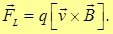
The force with which a magnetic field acts on a particle moving with velocity v and carrying charge q is proportional to the magnitude of the magnetic field, that is, to the magnetic flux density vector B, to the velocity of the charge v, and to the magnitude of the charge q itself. Experiments have shown that this force is orthogonal both to the velocity of the charge and to the magnetic flux density vector. This force is called the Lorentz force, and it is defined by the vector (cross) product
|
|
(5.3) |
According to this expression, the Lorentz force is perpendicular to the plane containing the vectors v and B and is determined for a positive charge by the right-hand screw rule (Fig. 5.8).
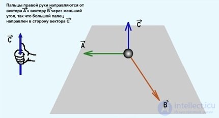
Fig. 5.8. The screw rule for determining the direction of the vector product
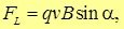
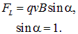
The magnitude of the Lorentz force is equal to
|
|
(5.4) |
where  — is the angle between the vectors v and B. The above relations can be used to measure the magnitude and direction of the magnetic flux density vector B, just as the relation

Is the definition of the electric field strength vector.
|
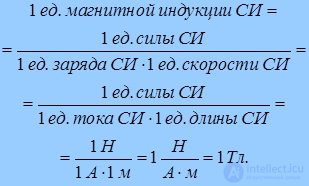
In the SI system, the unit of magnetic flux density is the tesla (T)
|
The tesla — is a large unit; magnets with a field of 10–8 T are considered record-setting.
Since the Lorentz force FL is always directed perpendicular to the velocity of the particle's motion v, it does no work. Consequently, the kinetic energy of a charged particle moving in a magnetic field does not change, and hence the magnitude of the particle's velocity does not change. The Lorentz force changes only the direction of the vector v, that is, it imparts a normal (centripetal) acceleration to the particle.
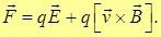
If a charge moves in a region where both an electric field E and a magnetic field B exist, then the total force acting on it is
|
|
(5.5) |
(This total force acting on a charge in an electromagnetic field is often what is called the Lorentz force).
The motion of charged particles in electric and magnetic fields underlies many phenomena occurring in the Universe. For example, charged particles of cosmic rays, interacting with the Earth's magnetic field, give rise to many interesting phenomena, including the polar auroras. The Earth's magnetic field is able to trap charged particles arriving from space near the Earth, and as a result the radiation belts surrounding the Earth arise (see Fig. 5.5).
The study of the motion of charged particles in electric and magnetic fields has made it possible to determine the specific charges of these particles (that is, the ratios of charge to mass) and thereby obtain valuable information about the nature of the particles and the processes in which they arise.
The action of electric and magnetic fields on beams of electrons and other charged particles is used to control these beams, which underlies various physical devices ranging from cathode-ray tubes to the most modern charged-particle accelerators.
Figure 5.9 shows an experiment demonstrating the deflection of an electron beam in a cathode-ray tube (Fig. 5.10) under the action of the Lorentz force arising when a permanent magnet, shaped as a long cylinder, is brought close to the tube. It is shown that the force is perpendicular to both the direction of the current in the beam and the direction of the magnetic field, and reverses sign when the direction of the magnetic field is reversed.
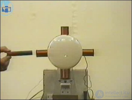
Fig. 5.9. Deflection of an electron beam in a cathode-ray tube under the action of the Lorentz force
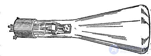
Fig. 5.10. Cathode-ray tube with deflecting plates and coils
Figure 5.11 shows the experiment of De la Rive, in which the action of a magnetic field on an arc discharge in a rarefied gas is observed. The gas is contained in a bulb, into which the cylindrical end of an electromagnet core is inserted. The discharge occurs between an electrode at the top of the bulb and a ring at the bottom encircling the core. After the magnetic field is switched on, the discharge cord between the upper electrode and the ring begins to rotate around the core under the action of the Lorentz force, and when the direction of the magnetic field is reversed, the direction of rotation of the cord reverses as well.
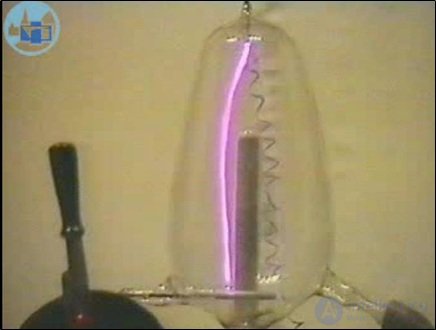
Fig. 5.11. De la Rive's experiment
Examples of magnetic fields encountered in our world are shown in Fig. 5.12.
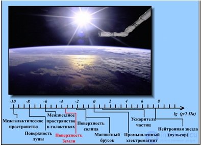
Fig. 5.12. Characteristic magnetic fields found in nature
If the initial velocity of a charged particle v is perpendicular to the magnetic field B, then in this case, under the action of the Lorentz force, the particle will move in a circle of constant radius R (Fig. 5.13)
|
|
(5.6) |
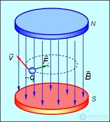
Fig. 5.13. Motion of a negatively charged particle in a uniform magnetic field
The Lorentz force FL, directed along the radius toward the center of the circle, produces a radial (centripetal) acceleration. By Newton's second law we have
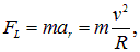
hence we can write the equation
|
|
(5.7) |
from which we can easily obtain an expression for the angular velocity of the particle
|
|
(5.8) |
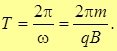
If q, m, and B are constant quantities, then the angular velocity, and consequently the period,
|
|
(5.9) |
are also constant quantities, independent of the particle's energy. Only the radius of the orbit depends on the particle's speed
|
|
(5.10) |
The Lorentz force produces only normal (centripetal) acceleration and is accordingly directed toward the center of the circle. Consequently, the direction of rotation of a positively charged particle is such that a screw rotating in the same direction would advance opposite to the direction of the field. A negatively charged particle rotates in the opposite direction (see Figs. 5.14, 5.15).
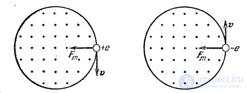
Fig. 5.14. Motion of positively and negatively charged particles in a uniform magnetic field.
The direction of the magnetic field is indicated by dots
If the initial velocity of a particle is parallel to the magnetic flux density vector, the Lorentz force is zero. The particle will continue to move in the same direction, in a straight line and at a constant speed.
Finally, in the general case we can imagine a particle entering a region of uniform magnetic field with velocity v, making an angle q with the direction of the magnetic field. This velocity can be resolved into two components, one of which

is directed along the field, while the other

is perpendicular to the field. Accordingly, the motion of the particle is the sum of two motions: uniform motion along the field with speed  and rotation in a circle with angular velocity
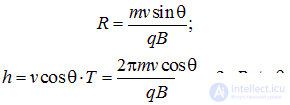
  . The particle's trajectory is thus a helix with radius R and pitch h (Fig. 5.15):
|
|
(5.11) |
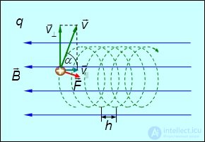
Fig. 5.15. Motion of a charged particle along a helix in a uniform magnetic field
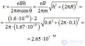
Example. A proton moves in a uniform magnetic field with an induction of 2 T. Its trajectory is a helical line with a radius of 10 cm and a pitch of 60 cm. Find the speed and kinetic energy of the proton. What accelerating potential difference U did the proton pass through before entering the magnetic field?
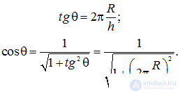
Solution. From equations (5.11) we find the angle between the proton's velocity and the field
|
|
(5.12) |
from which
|
|
(5.13) |
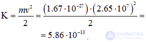
The kinetic energy of the proton will be
|
|
(5.14) |
We could use the nonrelativistic formula for the energy, since the speed of the proton is much less than the speed of light.
If the proton was accelerated by an electric field, then upon passing through a potential difference U it acquired energy eU. From this we find the potential difference
|
|
(5.15) |
The joule — is too large a unit of energy in the world of elementary particles. Here a non-SI unit is used — the electron-volt (eV).
|
An electron-volt (eV) — is a non-SI unit of energy numerically equal to the energy acquired by an electron passing through an accelerating potential difference of 1 V
|
It is convenient in that any other particle whose charge magnitude equals the charge of the electron, accelerated through a potential difference of 3.66 MeV, as in our example, has a kinetic energy of 3.66 MeV (megaelectron-volts).
The Cyclotron
The independence of the period of revolution of a nonrelativistic charged particle in a uniform magnetic field from its speed is the basis of a charged-particle accelerator called the cyclotron. In a cyclotron, a charged particle, placed between the poles of an electromagnet, repeatedly passes through an electric field, each time increasing its energy by an amount ranging from several hundred to several thousand electron-volts. As the particle's speed increases (as its energy grows), the radius of the orbit increases, so the particle in a cyclotron moves along a spiral. The cyclotron consists of two electrodes shaped like the halves of a low, round box (Fig. 5.16).
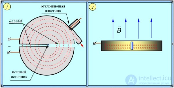
Fig. 5.16. Diagram of a cyclotron: 1 — top view; 2 — side view
The electrodes are called dees because of the resemblance of their shape to the capital Latin letter D. The dees are enclosed in an evacuated housing (vacuum of 10–5 mm Hg), which is placed between the poles of a large electromagnet. The field created by the electromagnet is uniform and perpendicular to the plane of the dees. An alternating voltage, produced by a high-frequency generator, is applied to the dees. Near the center of the magnet, in the gap between the dees, is located a source of charged particles — ions. A positive ion emitted from the source at a time when electrode 2 has a negative potential acquires some speed and, inside dee 2, describes a semicircle of constant radius, since inside the dee there is no electric field, only a magnetic field. By the time the ion leaves dee 2, the high-frequency generator reverses the direction of the electric field: dee 1 acquires a negative potential, and dee 2 a positive one. The ion is therefore accelerated again and, inside dee 1, describes a semicircle of a now larger radius (but the time taken to traverse the semicircle remains unchanged!). Moving in resonance with the high-frequency field, the ions spiral outward toward the edge of the magnet, their energy increasing after each passage of the particle through the accelerating gap between the dees. The beam of accelerated ions leaves the cyclotron by means of a deflecting electrode, to which a high negative potential is applied.
Figure 5.17 shows cyclic charged-particle accelerators.
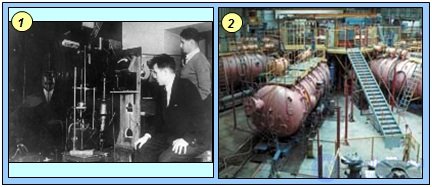
Fig. 5.17. Cyclic accelerators of elementary particles:
1 — the first Soviet cyclotron (1935);
2 — a modern cyclotron for research in controlled thermonuclear fusion
The cyclotron is used as an accelerator for heavy elementary charged particles and multiply charged positive ions. There are reasons of a fundamental nature that limit the possibility of significantly increasing the energy of ions in a cyclotron. The period of revolution in a cyclotron is proportional to the mass of the particle

However, in accelerators where particles are accelerated to speeds close to the speed of light, the relativistic expression for the particle's momentum must be taken into account. Then the equation of motion takes the form
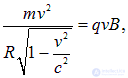
from which we obtain for the radius of the orbit
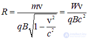
Here we have used the expression for the relativistic energy W of the particle
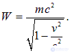
We then find for the period of revolution
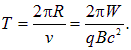
At small kinetic energies

and we return to the earlier formula. However, as the particles are accelerated, the period of revolution grows together with the energy, whereas the period of the high-frequency field in the cyclotron does not change. As a result, on each successive pass through the accelerating gap the particles fall increasingly behind, acquiring less and less energy, until they begin to enter the decelerating phase of the field. Therefore, two methods are used to achieve higher particle energies:
Determination of the Charge and Mass of the Electron
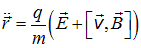
The equation of motion (Newton's second law) of a particle of mass  with charge
  , moving in an electromagnetic field, has the form
|
|
(5.16) |
It can be seen that, for any field configuration, the charge and mass enter only as the ratio — the specific charge  . Therefore, by measuring the parameters of the trajectory of a charged particle in an electromagnetic field, one can determine precisely its specific charge (Fig. 5.18). It remains to create a field configuration convenient for measurement.
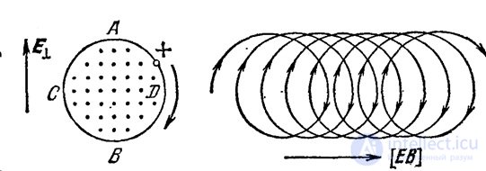
Fig. 5.18. Trajectory of a charged particle in crossed electric and magnetic fields
Consider a charged particle moving in space with velocity  and entering a uniform electric field perpendicular to the direction of its motion

where the field region has an extent l1 (Fig. 5.19).
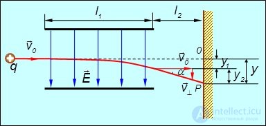
Fig. 5.19. Motion of a charged particle in a deflecting electric field
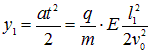
In the absence of the field  the particle would strike point 0 on the screen. In the field, however, a force F acts on the particle, directed perpendicular to the velocity v0, causing the particle to acquire an acceleration a = (q/m)E, where q/m is the specific charge of the particle. During the time it takes to traverse the field region

the particle is displaced vertically by a distance
|
|
(5.17) |
and acquires a velocity component perpendicular to the direction of the initial velocity v0
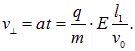
Further on, the particle, having left the region of the field, moves freely, with a velocity

directed at an angle  to the original one, where
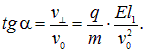
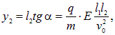
During the time it takes to reach the screen, the particle manages to shift by an additional distance
|
|
(5.18) |
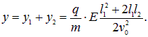
(see Fig. 5.19). It ultimately strikes point P on the screen, located at a distance from point 0 equal to
|
|
(5.19) |
The results obtained allow us to draw the following conclusions:
In 1897, J. J. Thomson was the first to determine the specific charge of the electron e/m along essentially this scheme, using a gas-discharge tube (Fig. 5.20). The electron beam passed through a hole in the anode and entered a region containing a uniform electric field from a capacitor and a magnetic field perpendicular to it, produced by a current-carrying coil (in Fig. 5.20 the region of the magnetic field is shown by a dotted line).
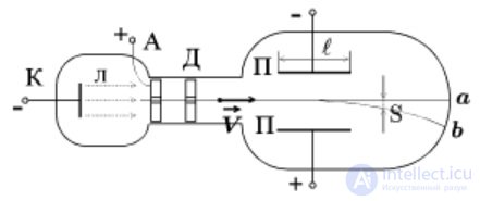
Fig. 5.20. The gas-discharge tube used to determine the specific charge of the electron
With the field switched off, the electron beam, moving in the direction of its initial velocity v0, produced a glowing spot at point 0 on the fluorescent screen. Switching on the magnetic field caused the glowing spot on the screen to shift. Then, by adjusting the magnitude of the field strength E of the capacitor's electric field, it was possible to arrange for the electron beam not to shift relative to point 0. In this case the effects of the electric and magnetic fields on the electrons cancelled each other out, that is, the following condition was satisfied (in (5.20) it is taken into account that  )
)
|
|
(5.20) |
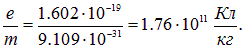
Knowing the field strengths, it was possible to determine the speed of the electrons v0 = E/B. By varying the fields and measuring the displacement of the glowing spot on the screen, the specific charge of the electron was determined from the speed of the electrons and the geometric dimensions of the setup. Thomson obtained
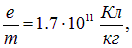
the modern value
Mass Spectrometers
To determine the specific charge, instruments called mass spectrometers or mass spectrographs are also widely used. The difference in the names of these instruments is related to the different methods of registering ions: by means of electronic circuits (mass spectrometers) or by means of photographic plates (mass spectrographs).
Various types of these instruments are based on the use of the focusing properties of electric and magnetic fields with respect to charged particles. Charged particles (ions or nuclei) are accelerated by an electric field (Fig. 5.21).
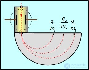
Fig. 5.21. Diagram of the operation of a mass spectrograph
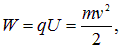
After passing through a potential difference U, the kinetic energy of the particles is equal to
|
|
(5.21) |
where q = Ze is the charge of the ion (or nucleus), m is the mass of the ion, and v is its speed. Entering a vacuum chamber with a uniform magnetic field of flux density B, perpendicular to the initial velocity, the particles describe a semicircle (under the influence of the Lorentz force). The radius of the circle along which the ion moves in the magnetic field is found from the condition
|
|
(5.22) |
Having traced a semicircle, the ions strike a photographic plate at a distance of 2R from the slit. Solving equations (5.21) and (5.22) together, we obtain
|
|
(5.23) |
Consequently, ions of each kind (determined by the value of q/m), depending on the magnitude of the deflecting magnetic and accelerating electric fields, strike the photographic plate at a certain definite location, characterized by the value of the radius R. Knowing the parameters of the instrument, the values of B and U, one can find the specific charges of the ions.
In 1880, E. Hall discovered that in a conductor placed in a magnetic field, a potential difference arises in the direction perpendicular to the magnetic flux density vector B and the current I. This is explained by the action of the Lorentz force on the charges moving in the conductor.
Figure 5.22 shows a conducting plate pierced by a magnetic field of flux density B, directed perpendicular to the drawing, away from us (indicated by a cross).
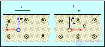
Fig. 5.22. For a fixed direction of the current, the Lorentz force
acting on the charge carriers in a sample placed in a magnetic field
has the same direction regardless of the sign of the carrier's charge
For negative charges, the velocity vector v and the current I point in opposite directions, while for positive charges the directions of velocity and current coincide. Applying the right-hand screw rule, we find that the Lorentz force in both cases is directed toward the upper face of the plate. Consequently, the charge carriers, regardless of the sign of their charge, accumulate on the upper face of the plate.
The Hall effect is observed in metals and semiconductors. In metals and in n-type semiconductors, where the charge carriers are electrons, excess negative charges accumulate on the upper face of the plate, while the lower face becomes positively charged (Fig. 5.23). In p-type semiconductors, where the carriers are so-called holes, which carry a positive charge, the upper face becomes positively charged and the lower one — negatively.
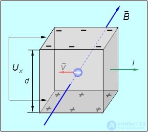
Fig. 5.23. The Hall effect consists in the appearance of a potential difference UX,
between the faces of a current-carrying conducting plate placed in a magnetic field
(the signs of the charges are shown for a metal plate)
Since

the Lorentz force is equal to
|
|
(5.24) |
The charges accumulated on the upper and lower boundaries of the plate create an electric field of strength EX , which in turn acts on the electric charges with a force
|
|
(5.25) |
When a steady-state distribution of charges is established in the cross-section of the conductor, these two forces balance each other

that is

from which
|
|
(5.26) |
Note that here the relation between the velocity of the charges and the fields EX and B is automatically satisfied, which we have just encountered while discussing Thomson's experiments on measuring the specific charge of the electron. When relation (5.26) is satisfied, the charge moves in a straight line at constant speed in crossed electric and magnetic fields.
From the formula for the current density j = qnv we find the drift speed of the charges
|
|
(5.27) |
Thus, for the strength of the transverse (Hall) electric field we obtain
|
|
(5.28) |
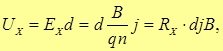
Consequently, for a distance d between the faces of the plate, the potential difference between them is equal to
|
|
(5.29) |
where RX = 1/qn — is the proportionality coefficient called the Hall constant. The density of charge carriers (electrons) in a metal is n = 1028 m–3, whence RX = 10–9 m3/C. For the most common semiconductors
RX = 0.1 m3/C.
The Hall effect is one of the effective methods for studying the properties of charge carriers in metals and semiconductors. Fig. 5.24 shows an experiment demonstrating the appearance of a transverse emf when a current-carrying semiconductor is placed in a magnetic field perpendicular to the current. A flat semiconductor sample, mounted on a holder, is introduced into the field of a permanent magnet, and a voltmeter registers the presence of the Hall emf. When the sample is flipped relative to the field, the sign of the emf reverses.
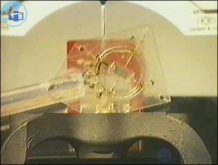
Fig. 5.24. The Hall effect in a semiconductor
Now we are ready to discuss the interaction of a current with a magnetic field.
Ampère established the existence of a force interaction between two conductors carrying electric currents. Let there be two long parallel conductors (Fig. 5.25-1).
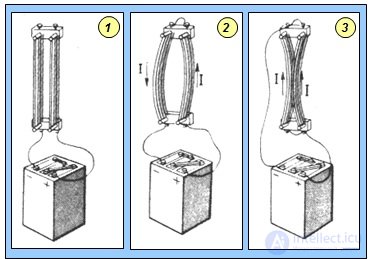
Fig. 5.25. Ampère's experiment studying the interaction of parallel currents:
1 — setup diagram; 2 — repulsion of antiparallel currents; 3 — attraction of parallel currents
If currents flowing in opposite directions are passed through them, the conductors will repel each other (see Fig. 5.25-2). If, however, the currents flow in the same direction, they will attract each other (see Fig. 5.25-3).
Video 5.4. Interaction of parallel currents.
Experiments conducted by Ampère showed that a force acts on a current-carrying conductor placed in a magnetic field. Where does it come from? In discussing the Hall effect, we saw that the electric field force EX balances the Lorentz force acting on the electrons. But the Hall field EX also acts on the crystalline ion lattice of the substance. In Fig. 5.23 the field EX is directed upward, orthogonal to the current and the magnetic induction. The force acting on the conductor will be directed the same way. Let us find its magnitude. If the cross-sectional area of the conductor is S, and its length (in the direction of the current) — dl, then in the given volume dV = dl · S there are dN = ndV = n · dl · S conduction electrons. Their total charge equals dQ = edN = en · dl · S. Owing to the overall neutrality of the conductor, the total charge of the ions of the crystal lattice has the same absolute value. Using formula (5.28), we find the total force acting on the crystal lattice framework of the section of conductor in question
|
|
(5.30) |
where we expressed the current density through its current strength

Note that this formula does not include the characteristics of the specific charge carriers, but only the total current through the conductor.
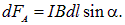
In our case the external magnetic field was orthogonal to the current. In the general case we shall characterize the direction of the current by the vector dl, having length dl and directed along the flow of the current. Only the component of the magnetic field orthogonal to the vector dl contributes to the Hall electric field strength. This component is equal in magnitude to

where is the angle between the vectors B and dl. Then for the magnitude of the force we have
|
|
(5.31) |
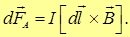
Taking into account the direction of this force (the screw rule), we can write it in vector form
|
|
(5.32) |
Expression (5.32) is called Ampère's law, and the force  is called the Ampère force (Fig. 5.26).
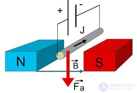
Fig. 5.26. The Ampère force acting on a current-carrying wire in the field of a permanent magnet
Video 5.5. The Ampère force: a wire jumping out of a magnet.
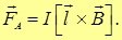
We have obtained an expression for the force acting on an element dl of the conductor. To determine the total force acting on the conductor, we must integrate (5.32) along its length, taking into account the dependence of the magnetic field on the position of the element. Such integration becomes trivial for a straight conductor in a uniform magnetic field
|
|
(5.33) |
The direction of the Ampère force is determined by the left-hand rule (Fig. 5.27):
|
If the left hand is positioned so that the lines of magnetic induction enter the palm, and the outstretched fingers point in the direction of the current, then the bent thumb shows the direction of the Ampère force acting on the conductor. |
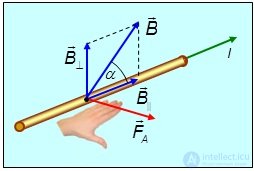
Fig. 5.27. Determining the direction of the Ampère force
Video 5.6. The Ampère force: Eichenwald's cart.
The action of the Ampère force on a current-carrying conductor is demonstrated in the experiment shown in Fig. 5.28. Horizontal conducting rails, along which an aluminum tube can roll, are placed on the end face of a vertical cylindrical coil. After the current through the coil is switched on, a constant voltage is applied to the rails, and a current begins to flow through the tube. Under the action of the Ampère force, the tube rolls along the rails. When the direction of the current in the tube is reversed, it rolls in the opposite direction.
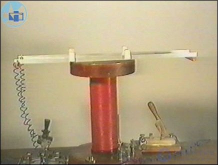
Fig. 5.28. Experimental study of the Ampère force
In the general case of an arbitrary conductor and magnetic field, the forces acting on different elements of the conductor differ in both magnitude and direction (Fig. 5.29).
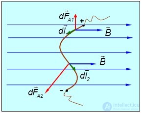
Fig. 5.29. In the general case, the forces acting on different elements of a conductor
differ in both magnitude and direction
With the help of formula (5.31) one can determine the magnitude of the magnetic induction from the maximum Ampère force dFA (in this case  ), acting on an element dl of a conductor carrying current I

That is, the magnitude of the magnetic induction is numerically equal to the maximum force acting on a unit element of current.
Let a current loop be placed in a magnetic field, and let it be able to rotate about the vertical axis OO' (Fig. 5.30-1). The Ampère forces acting on the sides of the loop of length l are perpendicular to them and to the magnetic field, and are therefore directed vertically: they only deform the loop, tending to stretch it. The sides of length a are perpendicular to B, so that a force F = BIa acts on each of them. These forces tend to turn the loop so that its plane becomes orthogonal to B.
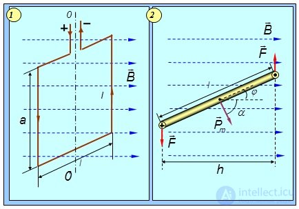
Fig. 5.30. Forces acting on a current loop in a magnetic field:
1 — side view; 2 — top view (scale enlarged)
Video 5.7. A current loop in a uniform magnetic field.
Video 5.8. A current loop in a non-uniform magnetic field.
The moment of the couple (Fig. 5.30-2) equals
|
|
(5.34) |
where  — is the arm of the couple, and
  — is the angle between the vector B and the side l.
|
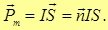
The quantity numerically equal to the product of the current I flowing in the loop and the area of the loop S = al is called the magnetic moment Pm of a flat current loop
|
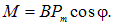
Thus, we can write the moment of the couple in the form
|
|
(5.36) |
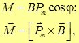
The magnetic moment of a current loop is a vector quantity. The direction of Pm coincides with the positive direction of the normal to the plane of the loop, which is determined by the screw rule: if the handle is rotated in the direction of the current in the loop, the translational motion of the screw shows the direction of the vector Pm . Let us introduce into formula (15.36) the angle a between the vectors Pm and B. The following relation holds
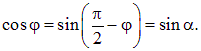
Hence,
|
|
(5.37) |
that is, the torque  , acting on a current loop in a uniform magnetic field, equals the vector product of the magnetic moment
  of the loop and the magnetic induction vector
  (Fig. 5.31). At
  the magnitude of the torque is maximal

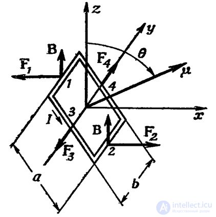
Fig. 5.31. Forces acting on a rectangular current loop in a magnetic field.
The magnetic field is vertical, and the magnetic moment is perpendicular to the plane of the loop
Video 5.9. A current loop in a magnetic field: model of an electric motor.
Once again the analogy with electrostatics is transparent: when discussing the electric dipole, we obtained an expression for the torque acting on it from the electric field in the form
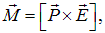
where  — is the electric dipole moment.
|
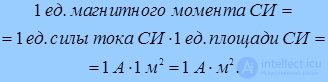
In the SI system, the unit of measurement of the magnetic moment of a loop is the ampere per square meter (A · m2)
|
Video 5.10. «Conscious coils»: repulsion and attraction of parallel currents and the rotation of the magnetic moment along the magnetic field.
Example. A current of 100 A flows through a thin wire in the form of a ring of radius 30 cm. A uniform magnetic field with a magnetic flux density of 20 mT is set up perpendicular to the plane of the ring (Fig. 5.32). Find the force stretching the ring.
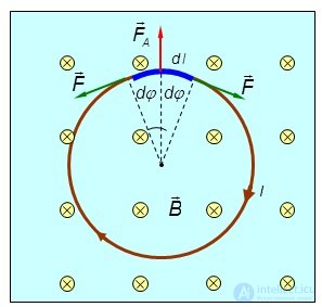
Fig. 5.32. Forces stretching a current-carrying ring in a magnetic field
Solution. Let the magnetic field be directed away from us, behind the plane of Fig. 5.32 (shown by crosses), with the current flowing clockwise. Let us select an element of length dl, subtending an angle  as seen from the center. An Ampère force
  acts on this element, directed along the radius of the ring. In addition, because of the stretching of the ring, tension forces F act on the ends of the element, and it is these that we need to find in the problem. The projection of these forces on the radial direction equals

Equating this projection to the Ampère force, we find













Comments