
Lecture
We are beginning the shortest chapter of this course. This material has been separated into its own chapter due to its importance and to summarize what we have learned about the fundamentals of electrical and magnetic phenomena. For simplicity we will consider fields in vacuum.
So, let us fix what we have already learned. All our formulas can be derived from a few statements.
Statement 1.
|
An electrostatic field is created by charges. The lines of force of an electric field begin and end on charges. |
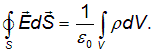
The mathematical formulation of this statement is the Ostrogradsky — Gauss theorem for the electric field strength
|
|
(9.1) |
On the right-hand side stands the integral of the charge density over an arbitrary volume, which equals the total charge inside it. On the left-hand side — the flux of the electric field strength vector through an arbitrary closed surface bounding this volume. As we have seen, Coulomb's law is also contained in this equation.
Statement 2.
|
Magnetic charges do not exist in nature. |
The mathematical formulation of this statement is the Ostrogradsky — Gauss theorem for the magnetic flux density vector, on the right-hand side of which stands zero
|
|
(9.2) |
Statement 3.
|
An electrostatic field is potential: it has no closed lines of force. |
Mathematically this is expressed as the equality to zero of the circulation of the electrostatic field strength along an arbitrary loop
|
|
(9.3) |
Statement 4.
|
A curl (vortex) magnetic field is created by electric currents. |
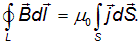
The mathematical expression of this statement is the circulation theorem for the magnetic flux density vector
|
|
(9.4) |
On the left-hand side stands the circulation of the magnetic field along an arbitrary loop L, and on the right-hand side — the integral of the total current density over an arbitrary surface S spanning this loop. This integral equals the sum of the currents crossing the surface S. The Biot — Savart — Laplace law is contained in this equation.
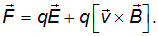
These four equations must be supplemented with the expression for the Lorentz force acting on moving charges from electromagnetic fields
|
|
(9.5) |
The attentive reader will notice that the headings of the last two statements are set in a different typeface. This is not by chance: these statements are subject to modification. The fact is that since we formulated these four statements, we have become acquainted with one more phenomenon — electromagnetic induction. It has not yet found reflection in the equations written out. Let us do this now.
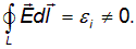
If the magnetic flux through a conducting loop L changes, then an induced emf arises in the loop. What does this mean? Charges located in the conductor will experience the action of a force associated with this emf. But the appearance of a force acting on a charge means the appearance of some electric field. The circulation of this field around the loop is, by definition, exactly equal to the induced emf
|
|
(9.6) |
The fact that the circulation is nonzero means that this electric field is not potential but has a curl (vortex) character, similar to the magnetic field. But if such a field has appeared, then what is the role of the loop? The loop — is nothing more than a convenient detector for registering the curl electric field via the induced current that arises. In order to dispense with the loop entirely, let us express the induced emf in terms of the magnetic flux. Let us rewrite Faraday's law in the form
|
|
|
|
Combining this equation with (9.6), we arrive at the modified statement 3 (Fig. 9.1).
Statement 5.
|
A time-varying magnetic field gives rise to a curl electric field. |
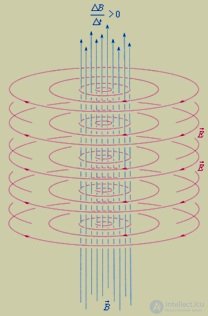
Fig. 9.1. The law of electromagnetic induction in Maxwell's interpretation:
a changing magnetic field generates a curl electric field
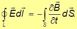
Mathematically this is expressed as the equation
|
|
(9.7) |
Faraday's law of electromagnetic induction is contained in this equation.
Here we must exercise a bit of caution: since we now have an additional electric field, will it not change the first statement? Fortunately, the answer is no: the flux of the curl field through a closed surface is equal to zero, so this field will not contribute to the left-hand side of equation (9.1).
It would seem that we have already accounted for all the phenomena we are familiar with. Why then did we mark the fourth equation as requiring modification? The fact is that now the symmetry between electric and magnetic phenomena is broken. Suppose that there are neither charges nor currents in the system. Can an electromagnetic field exist in that case? We know the answer from modern life: it can! Electromagnetic waves do exist, propagating through space and requiring no medium to do so. In the absence of charges and currents, the first two equations (9.1) and (9.2) are fully symmetric. The same cannot be said of the second pair of equations. Can an electric (curl) field be produced without charges, simply by changing the magnetic field? Why then can a magnetic field not be produced not by currents, but by changing the electric field?
J.C. Maxwell (Fig. 9.2) was the first to ask the question of modifying the fourth statement. No experimental facts pointing to this were known at the time. It follows from the fourth statement that the currents generating the curl magnetic field must be closed; they cannot be interrupted anywhere. Indeed, one can span a single loop L with many surfaces S. Suppose, say, we choose two of them — S1 and S2. Since the left-hand side of (9.4) is the same for them, the right-hand sides must also be equal. This means that all the current entering through S1 must exit through surface S2. This is indeed what happens with ordinary currents. But there are non-stationary cases where the electric charge density changes at some points. The current lines will then end at those points, which contradicts (9.4).
Fig. 9.2. J.C. Maxwell (1831–1879) — English physicist and mathematician
To illustrate such cases, let us consider the already familiar process of a capacitor discharging. Suppose there are two plates with charges +q and –q. As long as the circuit is open, the equal and opposite charges create a constant electric field in the space between the plates. No current flows through the wires, and there is no magnetic field around the circuit (Fig. 9.3-1).
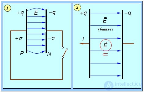
Fig. 9.3. Displacement currents in a capacitor: 1 — the initial state of the capacitor, 2 — the field changing during discharge. The time derivative of the electric field strength points in the same direction as the current density vector, and is equal to it in magnitude
When the capacitor discharges through the conductor connecting the plates, a current will flow from P to N (Fig. 9.3-2). A decrease in the charge on the plate by an amount dq means that this same amount of electricity will flow through the wire connected to the plate (conservation of charge).
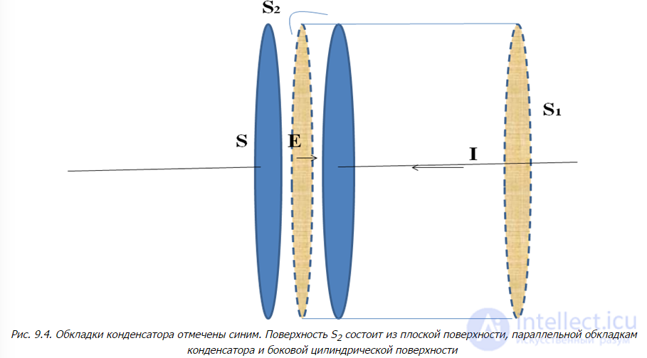
Fig. 9.4. The capacitor plates are marked in blue. The surface S2 consists of a flat surface parallel to the capacitor plates and a lateral cylindrical surface
We have the equation,
|
|
(9.8) |
which we would like to check for consistency.
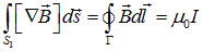
Let us integrate it over the surface S1 (Fig. 9.4). We get
|
|
(9.9) |
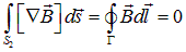
From this equality one usually obtains the value of the magnetic field B for an infinitely long conductor. Recall that the surface over which the integration is carried out can have any shape, provided that it is bounded by the loop G. Let us make use of this and integrate this same equation (9.8) over the surface S2. We get
|
|
(9.10) |
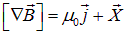
Here edge effects are neglected. The integral over the lateral (cylindrical) surface is equal to zero if the radius of the cylinder is chosen large enough. Expressions (9.9) and (9.10) contradict each other. This means that equation (9.8) is incorrect and must be changed. The simplest way — is to add to the right-hand side of equation (9.8) an unknown vector, which we shall denote 
|
|
(9.8a) |
Let us find the unknown vector , assuming that it is nonzero only between the capacitor plates. To do this we integrate separately over the surfaces S1 and S2 and equate the results. The integral over S1 was computed in (9.9), and the integral over S2 is
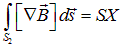
Equating:

So,

— together with (9.8a) we obtain Maxwell's equation
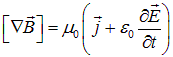
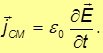
Maxwell called the quantity

the displacement current density:
|
|
(9.11) |
Since the numerical values of the displacement current density jdisp and the conduction current density j are equal, it follows that the lines of conduction current density inside the conductor continuously transform into lines of displacement current density between the plates (the capacitor plates).
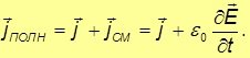
If we introduce the concept of the total current, which includes the sum of the conduction current and the displacement current, then for its density we have
|
|
(9.12) |
Using the example of the capacitor we found that the total current is closed: its lines continue without breaking anywhere (even in the space between the capacitor plates). Because of this property it is precisely the total current that must stand on the right-hand side of the equation (Fig. 9.5). This was Maxwell's idea.
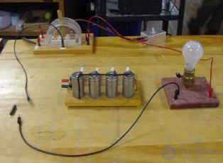
Fig. 9.5. A light bulb connected to an alternating-current mains through a capacitor
stays lit continuously, because the conduction current inside the conductor transforms into the displacement current between the capacitor plates
As a result we can formulate (Fig. 9.6)
Statement 4.
|
A curl magnetic field is created by the total current, that is, by the conduction current and the displacement current, caused by a changing electric field. |
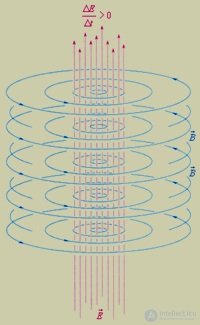
Fig. 9.6. Maxwell's hypothesis. A changing electric field gives rise to a curl magnetic field
The mathematical expression of this statement is the equation obtained from (9.11),
|
|
(9.13) |
Thus, Maxwell predicted a new phenomenon, in a certain sense the inverse of electromagnetic induction. Experiment confirmed that a magnetic field can indeed be created by a time-varying electric field (Fig. 9.7).
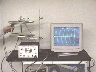
Fig. 9.7. An alternating electric field between the plates of a capacitor generates a curl magnetic field, which is measured using a square wire loop and displayed on a monitor screen
Among these experiments, the first and most important was the experimental proof of the existence of electromagnetic waves, carried out by the German physicist Heinrich Hertz in 1888 (Fig. 9.8). Interestingly, Hertz himself did not believe in their existence and, with his experiments, wanted to disprove Maxwell's theory, which he himself had created 20 years earlier, in 1865.
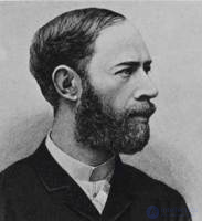
Fig. 9.8. Heinrich Hertz (1857 - 1894) - German physicist.
Hertz not only experimentally proved the existence of electromagnetic waves, but also was the first to study their properties — absorption and refraction in various media, reflection from metallic surfaces, and so on. He managed to measure experimentally the wavelength and propagation speed of electromagnetic waves, which turned out to equal the speed of light (Fig. 9.9).
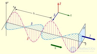
Fig. 9.9. A harmonic electromagnetic wave traveling along the z axis. The vectors of the electric field strength, the magnetic flux density, and the wave velocity are mutually perpendicular
Hertz's experiments played a decisive role in proving and gaining acceptance for Maxwell's electromagnetic theory. Seven years after these experiments, electromagnetic waves found application in wireless communication, demonstrated by A.S. Popov in 1895 (Fig. 9.10).
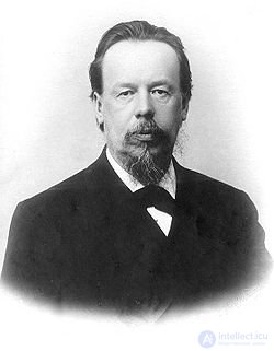
Fig. 9.10. A.S. Popov (1859–1905) — Russian physicist and electrical engineer
Electromagnetic waves can be excited only by accelerating charges. The simplest system that radiates electromagnetic waves is a small electric dipole whose dipole moment p(t) changes rapidly with time. Such an elementary dipole is called a Hertzian dipole. In radio engineering, the Hertzian dipole is equivalent to a small antenna whose size is much smaller than the wavelength λ (Fig. 9.11).
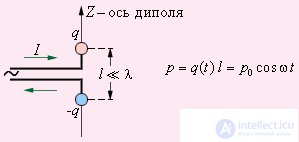
Fig. 9.11. An elementary electric dipole undergoing harmonic oscillations
Fig. 9.12 gives an idea of the structure of the electromagnetic wave radiated by such a dipole.
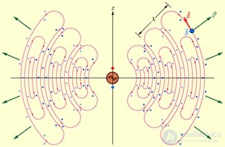
Fig. 9.12. Radiation from an elementary electric dipole. The dipole moment is directed along the z axis, the electric field lines lie in the plane of the page, and the magnetic field lines are perpendicular to the plane of the page
It should be noted that the maximum flux of electromagnetic energy is radiated in the plane perpendicular to the dipole axis. Along its axis, the dipole radiates no energy. Hertz used an elementary dipole as the transmitting and receiving antennas in the experimental proof of the existence of electromagnetic waves.
The four equations corresponding to our (modified) statements are called Maxwell's equations in integral form.
Let us write them all out together once again:
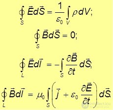
To obtain Maxwell's equations in a medium, one must make the substitution:
 ,
,
that is, specify the relation (the so-called «constitutive» equations) between the field strengths and the flux densities:  and
and  and supplement the system with the equation of Ohm's law
 .
.
Let us note that the simplest relations given above cannot always be used. The situation is noticeably more complex in the presence of substances such as ferroelectrics, piezoelectrics, ferromagnets, anisotropic media, and the like. Here our goal is to show how the complete system of equations is formed, which allows one (taking into account initial and boundary conditions, of course) to calculate the electromagnetic field.
From the equations in integral form one can pass, with the help of theorems of vector analysis, to the equations in differential form, relating the values of the fields  and
and  and their spatial and temporal derivatives to the values of the charge and current densities. We will not use these equations, but let us nevertheless give them, if only as part of a joke published in one of the journals on the days of Maxwell's anniversary:
«And God said:
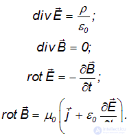
And there was light».
The unfamiliar symbols div (read as «divergence») and rot (read as «curl») — are special differentiation operations performed on vector fields. Divergence — from the Latin for «divergence, spreading apart». This operation describes a «hedgehog»-type configuration of field lines, diverging from points where electric charges are present. The word «curl» needs no translation, it is clearly associated with rotation. This operation describes vortex (curl) fields (ring-shaped — closed field lines) around their sources — currents or other fields changing in time.
The four integral equations and the four differential ones are equivalent. Maxwell showed that all phenomena of electromagnetism can be fully described by these four equations, which are a generalization of experimental facts.
In the joke given above, light was mentioned. Indeed, light — is electromagnetic radiation of a certain range of frequencies. The prediction of electromagnetic waves became one of the greatest achievements of Maxwell's theory. Let us imagine that charges and currents are absent. Let us look at Maxwell's equations in differential form. It can be seen that if the fields are not static but depend on time, then there is a curl electric and magnetic field (the corresponding curls are nonzero). The propagation of fields without charges and currents — is precisely electromagnetic waves. And one can discern in the equations a hint of their propagation speed: it involves the combination e0m0, through which the speed of light in vacuum can be expressed (see (6.3))

But more on that — later, in the next part of our course.
In conclusion of this part, let us quote the words of H. Hertz about Maxwell's equations:
«It is difficult to escape the feeling that these mathematical formulas have an independent existence and an intelligence of their own, that they are wiser than we are, wiser even than their discoverers, and that we get more out of them than was originally put into them».
Example of using Maxwell's equations
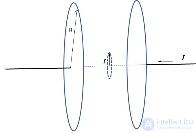
Determine the magnitude of the magnetic field in the gap of a capacitor as a function of r, the distance from the axis of symmetry (Fig. 9.13)
|
|
Fig. 9.13. A capacitor with circular plates in the process of charging
Solution
Let us write equation (9.13) for the loop shown in Fig. 9.3 with a dashed line. Integrating, we get
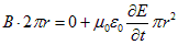
or

Obviously, the magnetic field is nonzero only because of the presence of an electric field changing with time. In turn, the change in the electric field is due to the increasing charge on the capacitor plates. We obtain this relation from the expressions

Finally we find

According to the formula obtained,

which is clearly incorrect. What is the mistake?
ANSWER: the formula is valid only for  .
.






Comments