
Lecture
|
Electric current — is the ordered motion of charged particles. The direction of the current is taken to be the direction of motion of positive charges. |
Several types of electric current are distinguished. Suppose there is a macroscopic charged body (for example, a sphere) that is moving through space. Since charges move together with the body, a directed motion of charges arises, that is, an electric current. Such a current, associated with the motion of macroscopic bodies, is called a convection (transfer) current. If, inside some body, a number of charged particles move in an ordered manner because an electric field is created within it, then such a current is called a conduction current. For a conduction current to arise, the presence of free charge carriers is necessary.
In conductors, part of the valence electrons are not bound to specific atoms and can move freely throughout its volume. In the absence of an electric field applied to the conductor, such free electrons — conduction electrons — move chaotically, frequently colliding with ions and atoms, thereby changing their energy and direction of motion. Through any cross section of the conductor, just as many electrons pass in one direction as in the opposite direction. Therefore, there is no net transfer of electrons through such a cross section, and the electric current is zero. If, however, a potential difference is applied to the ends of the conductor, then under the action of the electric field forces the free charges in the conductor begin to move from the region of higher potential to the region of lower potential — an electric current arises. It has historically been established that the direction of the current is taken to be the direction of motion of positive charges, which corresponds to their transition from higher to lower potential.
Electric current is characterized by the current I (Fig. 4.1).
|
Current is a scalar quantity numerically equal to the charge transferred through the cross section of a conductor per unit time
|
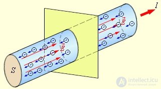
Fig. 4.1. Current in a conductor
According to (4.1), the current in a conductor equals the ratio of the charge  , passed through the cross section of the conductor over the time
  to this time.
Remark: In the general case, the current through a given surface equals the flux of charge through that surface.
If the current does not change with time, that is, if equal charges pass through any cross section of the conductor over any equal time intervals, then such a current is called direct (constant), and then the charge that has flowed over the time t can be found as (Fig. 4.2)
|
|
(4.2) |
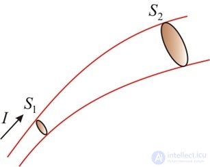
Fig. 4.2. Direct current flowing through different cross sections of a conductor
|
The quantity |
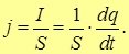
Taking into account the definition of current, the current density through a given cross section  can be expressed in terms of the current
  flowing through that cross section
|
|
(4.3) |
For a uniform distribution of charge flux over the entire cross-sectional area of the conductor, the current density equals
|
|
(4.4) |
|
In SI, the unit of current is the ampere (A). In SI, this unit is a base unit. |
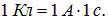
Equation (4.1) relates the units of current and charge
|
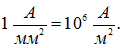
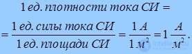
In SI, the unit of current density is the ampere per square meter (A/m2):
|
This is a very small quantity, so in practice larger units are usually used, for example
The current density can be expressed in terms of the volume charge density  and the velocity of their motion v (Fig. 4.3).
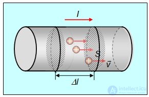
Fig. 4.3. On the relation of the current density j to the volume charge density  and the drift velocity v of the charge carriers. During the time dt all the charges from the volume dV = vdt S pass through the area S
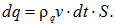
The total charge passing during the time dt through a certain surface S, perpendicular to the velocity vector v, equals
|
|
(4.5) |
Since dq/(Sdt) is the magnitude of the current density j, we can write
|
|
(4.6) |
Since the velocity v is a vector quantity, it is also convenient to regard the current density as a vector quantity, hence
|
|
|
|
Here  is the charge density,
  is the velocity of directed motion of the charge carriers.
Remark: For generality, the index  is used, since the charge carriers capable of participating in the formation of a conduction current can be not only electrons but, for example, protons in a beam obtained from an accelerator, or multiply charged ions in a plasma, or the so-called «holes» in «p»-type semiconductors, in short, any charged particles capable of moving under the action of external force fields.
In addition, it is convenient to express the charge density  in terms of the number
  of charge carriers per unit volume — (the concentration of charge carriers)
  . As a result we obtain:
|
|
(4.7) |
It should be emphasized that the current density, unlike the current, is a differential vector quantity. Knowing the current density, we know the distribution of the flow of charge over the conductor. The current can always be computed from its density. Relation (4.4) can be «inverted»: if we take an infinitesimally small element of area  , then the current through it is determined as
  . Accordingly, the current through any surface S can be found by integration
|
|
(4.8) |
What should be understood by the velocity of the charge v, if there are many such charges, and they certainly do not all move in the same way? In the absence of an external electric field, the thermal velocities of the current carriers  are distributed chaotically, obeying the general laws of statistical physics. The mean statistical value
  vanishes owing to the isotropy of the distribution over the directions of thermal motion. When a field is applied, a certain drift velocity arises — the mean velocity of the directed motion of the charge carriers:

which will be nonzero. Let us draw an analogy. When water gushes from a hose, and we are interested in how much of it arrives per unit time onto a flower bed, we need to know the speed of the jet and the cross-sectional area of the hose. And we are not at all concerned with the speeds of individual molecules, although they are very high, much higher than the speed of the water jet, as we established in the previous part of the course.
Thus, the velocity  in expression (4.7) — is the drift velocity of the current carriers in the presence of an external electric field or any other force field that causes directed (ordered) motion of the charge carriers. If charges of different sign can move in a substance, the total current density is determined by the vector sum of the charge flux densities of each sign.
As already noted, in the absence of an electric field, the motion of charge carriers is chaotic and does not produce a net current. If, by applying an electric field, we impart to the charge carriers even a small drift velocity (compared to their thermal velocity), then, owing to the enormous number of free electrons in conductors, a significant current arises.
Since the drift velocity of the current carriers is created by the electric field, it is logical to assume proportionality

so that the current density will also be proportional to the field strength vector (Fig. 4.4)
|
|
(4.9) |
This question is discussed in more detail in the Supplement
Included in relation (4.9)
|
The proportionality coefficient |
Conductivity relates the field strength at a given point to the steady-state «flow» velocity of the charge carriers. Therefore, it can depend on the local properties of the conductor near that point (that is, on the structure of the substance), but does not depend on the shape and size of the conductor as a whole. Relation (4.9) is called Ohm's law for the current density in a conductor (it is also called Ohm's law in differential form).
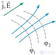
Fig. 4.4. The electric field lines coincide with the current lines
To get a sense of the orders of magnitude, let us estimate the drift velocity of charge carriers in one of the most common materials — copper. Let us take, for example, a current I = 1 A, and let the cross-sectional area of the wire be
1 mm2 = 10–6 m2. Then the current density equals j = 106 A/m2. Now let us use relation (4.7)

The charge carriers in copper are electrons (e = 1.6·10-19 C), and it remains for us to estimate their concentration  . In the periodic table, copper is placed in the first group of elements, it has one valence electron, which can be given up to the conduction band. Therefore, the number of free electrons approximately coincides with the number of atoms. We take from a reference the density of copper — r Cu=8.9·103 kg/m3. The molar mass of copper is given in the periodic table — MCu = 63.5·10–3 kg/mol. The ratio

— is the number of moles in 1 m3. Multiplying by Avogadro's number Na = 6.02·1023 mol–1, we obtain the number of atoms per unit volume, that is, the electron concentration

Now we obtain the sought estimate of the electron drift velocity

For comparison: the speeds of the chaotic thermal motion of electrons at 20°C in copper are of the order of magnitude of 106 m/s, that is, eleven orders of magnitude greater.
Let us take an arbitrary imaginary closed surface S, which is crossed in various directions by moving charges. We have seen that the total current through the surface equals
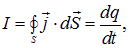
where dq — is the charge crossing the surface during the time dt. Let us denote by q ' the charge located inside the surface. It can be expressed in terms of the charge density  , integrated over the entire volume bounded by the surface
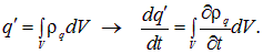
From the fundamental law of nature - the law of conservation of charge — it follows that the charge dq, that has left through the surface during the time dt, will decrease the charge q ' inside the surface by exactly this same amount, that is, dq ' = –dq or
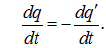
Substituting here the expressions written above for the rates of change of the charge inside the surface  , we obtain a mathematical relation expressing the law of conservation of charge in integral form
|
|
(4.10) |
Recall that the integrations are carried out over an arbitrary surface S and the volume V bounded by it.
Suppose that at the ends of a conductor of length l a potential difference 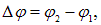 is created, which produces inside it an electric field E, directed toward the decrease of potential (Fig. 4.5-1). If the field inside the conductor can be considered uniform, then
|
|
(4.11) |
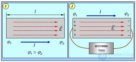
Fig. 4.5. A potential difference at the ends of a conductor is necessary for a current to arise.
A current source is needed to maintain the potential difference
In this case an electric current arises in the conductor, which flows from the higher potential  to the lower
  . The motion of (positive) charges from
  to
to  leads to the equalization of potentials at all points. The electric field in the conductor then vanishes, and the current ceases. Obviously, a necessary condition for the existence of a current is the presence of a potential difference

and to maintain it, a special device is needed by means of which the separation of charges at the ends of the conductor takes place. Such a device is called a current source. Thus, obtaining a current requires the presence of a closed circuit and a current source (Fig. 4.5-2). Galvanic cells, batteries, thermoelements, electric generators — are examples of current sources. A current source simultaneously performs a second task — it closes the electric circuit, along which the continuous motion of charges can take place. Current flows through the external part — the conductor, and through the internal part — the current source. A current source has two poles: a positive one, at a higher potential, and a negative one, at a lower potential. With the external circuit open, an excess of electrons forms at the negative pole of the current source, and a deficiency at the positive one. The separation of charges in the current source is carried out by means of external, so-called extraneous (external) forces, directed against the electric forces acting on charges of opposite sign in the conductors of the current source itself. The nature of the extraneous forces can be quite varied: mechanical, chemical (Fig. 4.6), thermal, biological, etc.
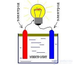
Fig. 4.6. The action of extraneous forces of chemical origin
Thus, the transfer of charge along a closed conductor under the action of a current source occurs owing to forces not of electrostatic origin — extraneous forces acting inside the source. Electrostatic forces cannot provide for the motion of charges around a closed loop because of their conservative nature (the work done by these forces around a closed loop is zero).
Thus, if a circuit consisting of a conductor and a current source is closed, then a current flows through it, and in the process work is done by the extraneous forces. This work consists of the work done against the forces of the electric field inside the current source  , and the work done against the mechanical resistance forces of the medium of the source
  , that is
|
|
(4.12) |
|
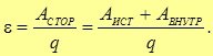
The ratio of the work done by the extraneous forces in moving a point charge along the entire circuit, including the current source, to the charge, is called the electromotive force (EMF) of the current source:
|
The work against the forces of the electric field equals
|
|
(4.14) |
If the poles of the source are open (no external circuit), then  , and then
|
|
(4.15) |
that is, the EMF of a current source with the external circuit open equals the potential difference produced at its poles.
The distribution of potential in a closed circuit is shown in Fig. 4.7.
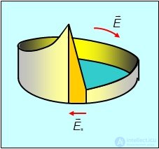
Fig. 4.7. Distribution of potential in a closed electric circuit
It is clear that positive charges move in the direction of decreasing potential. At the same time, there must be a region where the charges move in the direction of increasing potential owing to the extraneous forces. Put simply: for water to flow downhill, someone must first lift it up.
It was noted above (see (4.6)) that the current density j is proportional to the magnitude of the electric field E
|
|
|
(4.6) |
Why, then, did we assume that in conductors the mean velocity of the charges is constant and proportional to the magnitude of the electric field strength, rather than increasing without bound? Indeed, free charges outside a conductor, under the action of a uniform external field, would acquire an acceleration

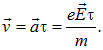
Thus, the directed velocity of the charges along the field (or against the field, if the charges are negative) would increase with time. Then the current density would also grow with time: j =  v = at. However, inside a conductor free charges undergo collisions with the atoms of the conductor. During the time of free flight t between two collisions, a charge in the conductor acquires a velocity along the external electric field
|
|
(4.16) |
After the next collision, the directed velocity is lost. Then, until the next collision, a new buildup of directed velocity takes place. Therefore, on average, the directed velocity of motion is constant and is determined by the velocity accumulated between two successive collisions.
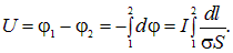
On a segment of a linear electric circuit of length dl, the field strength is related to the potential by the usual relation

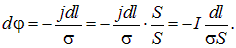
Consequently, we can write
|
|
(4.17) |
Video 4.1. Demonstration of the potential drop along a conductor carrying a current.
Here  and S — are the conductivity and the cross-sectional area of the conductor at the location where our chosen infinitesimal element dl is situated. But the current I will be constant along the entire length l of the conductor: for a stationary flow of charges, as many enter through one cross section of the conductor as leave through another. This is also a consequence of the law of conservation of charge and the assumed stationarity of the situation, in which, in particular,
  .
.
Owing to the current  being the same through any cross section of the conductor, when integrating relation (4.17) along the conductor from point 1 to point 2, we can take outside the integral sign:
|
|
(4.18) |
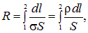
Under the integral sign is a quantity that does not depend on the magnitude of the current and the voltage at the ends of the conductor, but only on its geometric dimensions, shape, and material. It is called the resistance of the conductor between points 1 and 2
|
|
(4.19) |
where  — is the resistivity of the conductor.
Thus, we obtain

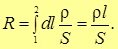
In the case of a straight, uniform conductor of constant cross section, its resistance will equal
|
|
(4.20) |
|
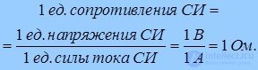
In SI, the unit of resistance is the ohm (Ω):
|
1 ohm — is the resistance of a segment of a circuit without an EMF, through which a current of 1 A flows when the voltage at its ends is 1 V (Fig. 4.8).
|
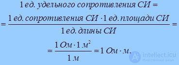
In SI, the unit of resistivity is the ohm · meter (Ω · m):
|
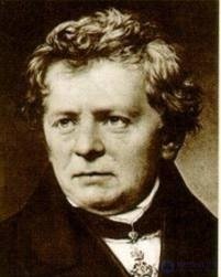
Fig. 4.8. G. Ohm (1787–1854) — German physicist
The resistivity  of a substance characterizes the conducting ability of the material, it is different for different substances and depends significantly on the temperature of the conductor. However, does not depend on the shape and dimensions of the conductor. We did not take outside the integral sign in (4.19) because there are circuits, individual sections of which are made of different materials. In this case, will depend on the integration variable
  . Values of the resistivity for some substances are given in the table.
Table
Resistivities of Some Conductors
|
Conductors |
Al |
Ag |
Cu |
Au |
W |
Fe |
Nichrome |
|
r (μΩ · m)
|
0.028 |
0.016 0.017 |
0.022 |
0.055 0.098 |
1.12 |
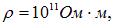
It is noteworthy that, overall, the resistivities of metals are close to one another, which testifies to a common conduction mechanism. The resistivities of poor conductors and insulators, on the other hand, vary over wide limits. For example, for sea water r = 0.3 Ω · m, for moist ground 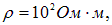 for glass
  for amber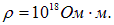
The relation obtained above
|
|
(4.21) |
is called Ohm's law in integral form (Fig. 4.9) for a uniform section of a circuit, that is, a section that contains no sources — no sources of extraneous forces, or simply Ohm's law (for such a section of a circuit).
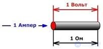
Fig. 4.9. Dimensions of physical quantities in Ohm's law
Example 1. A copper conductor has the shape of a truncated cone with base radii r1 = 1 mm and r2 = 2 mm. The length of the conductor is L = 10 cm. Find its resistance.
Solution. The dependence of the conductor's radius r(l) on the distance l, measured from the smaller base, is shown in Fig. 4.10.
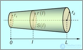
Fig. 4.10. On the calculation of the resistance of a conically shaped conductor
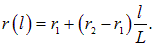
Mathematically, this dependence is expressed by the linear law
|
|
(4.22) |
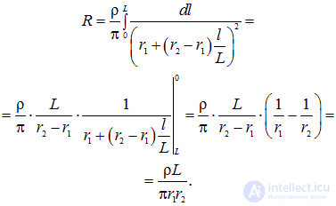
The cross-sectional area S(l) at a distance l from the left end can be found as
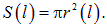
Then from formula (4.19) it follows that
|
|
(4.23) |
Substituting the numerical values, we find

In practice, electric circuits are an assembly of conductors connected to one another in a particular way. The series and parallel connections of conductors are the most common.
Series Connection of Conductors
|
A connection of conductors is called series (in series) if they are connected one after another in succession. |
In a series connection, according to the law of conservation of charge, the same charge passes through the resistors in the same time, so the currents in all the resistors are the same

The voltage drop across the first conductor is  across the second
  and so on (Fig. 4.11).
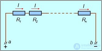
Fig. 4.11. Series connection of conductors
The sum of the voltage drops across all the resistors equals the voltage Uab at the ends of the circuit
|
|
(4.24) |
By Ohm's law for a segment of a circuit, we write
|
|
(4.25) |
Thus
|
|
(4.26) |
On the other hand, Uab = IRseries, where Rseries — is the total resistance of the circuit for a series connection. Consequently,
|
|
(4.27) |
Bringing together the relations obtained, we arrive at the law of series connection of conductors:
|
For a series connection of conductors: — the current is the same in all the conductors and equals the current in the entire circuit
— the voltage drop across the entire circuit equals the sum of the voltage drops across the individual conductors
— the resistance of the circuit equals the sum of the resistances of the individual conductors making up the circuit |
Parallel Connection of Conductors
|
A connection of conductors is called parallel if their beginnings are connected together and their ends are connected together. |
In a parallel connection (Fig. 4.12), the voltage Uab across the segment ab will be the same for each individual resistor, that is
|
|
(4.28) |
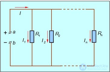
Fig. 4.12. Parallel connection of conductors
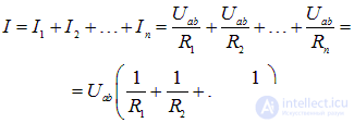
From the law of conservation of charge it follows that when a circuit branches, part of the charges may go along its individual sections, but the total amount of charge arriving at the branch point must equal the sum of all the charges leaving it. In other words, the current I equals the sum of the currents in the individual branches of the circuit
|
|
(4.29) |
On the other hand, the current over the entire segment equals
|
|
(4.30) |
where Rpar — is the total resistance of the circuit for a parallel connection.
Consequently,
|
|
(4.31) |
Bringing together the relations obtained, we arrive at the law of parallel connection of conductors:
|
For a parallel connection of conductors: — the voltage drop across each conductor is the same and equals the voltage drop across the entire circuit
— the current in the unbranched part of the circuit equals the sum of the currents in the individual conductors
— the resistance of the circuit equals
|
The formulas for series and parallel connection of conductors make it possible, in many cases, to calculate the resistance of a complex circuit consisting of many resistors. Fig. 4.13 shows an example of such a complex circuit and indicates the sequence of calculations.
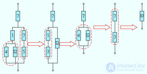
Fig. 4.13. Calculation of the resistance of a complex circuit. The resistances of all conductors are given in ohms (Ω)
Circuits like the one shown in Fig. 4.14, as well as branched circuits containing several sources, are calculated using Kirchhoff's rules.
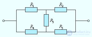
Fig. 4.14. An example of an electric circuit that cannot be reduced to
a combination of series- and parallel-connected conductors
As follows from (4.14), the work against the field forces inside the current source is expressed through the voltage drop across the external resistance R

For a closed electric circuit, the work against the resistance forces of the medium of the source  leads to a voltage drop
  inside the source, so that
|
|
(4.32) |
Ascribing to the current source an internal resistance r, we write the voltage drop across the internal segment of the circuit in accordance with Ohm's law
|
|
(4.33) |
As follows from (4.13), for a closed external circuit (Fig. 4.15, 4.16) the EMF of the current source e equals the sum of the voltage drops across the internal resistance of the source and across the external circuit
|
|
(4.34) |
whence
|
|
(4.35) |
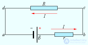
Fig. 4.15. The direction of the electric current J (1 → 2)
coincides with the direction of action of the current source with EMF e (3 → 4)
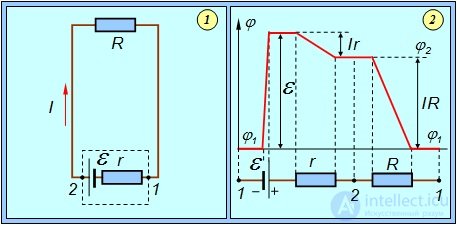
Fig. 4.16. A closed circuit with a resistive load R and a current source (shown by the dashed rectangle) with EMF e and internal resistance r. The voltage at the terminals of the source (points 1 and 2) equals  and is less than the EMF by the amount of the voltage drop Ir across the internal resistance. The distribution of potential along the circuit is shown on the right. The sum of the voltage drops across the internal resistance and the load (external circuit) equals the EMF of the current source
It can be seen that the external and internal resistances can be regarded as two resistances connected in series. Fig. 4.17 gives a schematic representation of a direct-current source with emf equal to  and internal resistance r in three regimes: «open circuit», operation under load, and short-circuit mode (s.c.). Shown are the field strength
  of the electric field inside the battery and the forces acting on positive charges:
  — the electric force and
  — the extraneous force. In short-circuit mode the electric field inside the battery vanishes.
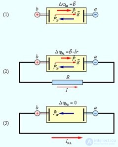
Fig. 4.17. Schematic representation of a direct-current source:
1 — battery open; 2 — battery closed onto an external resistance R; 3 — short-circuit mode
Measuring instruments — voltmeters and ammeters — come in two kinds: pointer (analog) and digital. Digital electrical measuring instruments are complex electronic devices. Digital instruments usually provide higher measurement accuracy (Fig. 4.18).
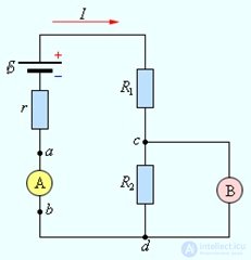
Fig. 4.18. Connecting an ammeter (A) and a voltmeter (V) into an electric circuit
Fig. 4.19 shows an experiment for studying the voltage drop across a section of a circuit. The voltage drop across a section of circuit containing an emf source depends on the current flowing through that section, and can even change sign when this current changes. This is demonstrated using a circuit in which two batteries, a rheostat, and an ammeter are connected in series. A voltmeter showing the voltage drop across one of the batteries is connected to it. As the current in the circuit is changed by means of the rheostat, the magnitude and sign of this voltage change.
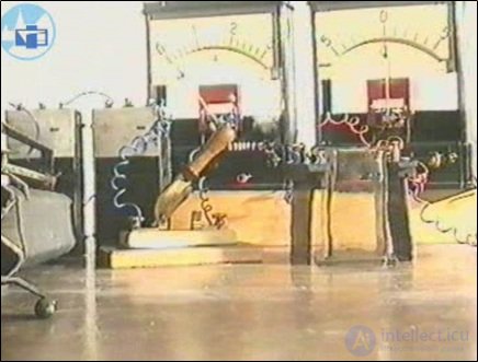
Fig. 4.19. Experiment for studying the voltage drop across a section of a circuit
In this section we shall solve problems on charging and discharging a capacitor. The electric circuit is shown in Fig. 4.20. The switch S allows the current source to be connected and
продолжение следует...
Часть 1 Direct electric current: current, voltage, emf, laws and rules
Часть 2 4.5. Kirchhoff's rules - Direct electric current: current, voltage, emf,


 , numerically equal to the charge passing through a unit area of the cross section of a conductor per unit time, is called the current density.


 is called the conductivity of the conductor material.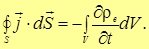























Comments