7. Heat capacity of crystals. Quantum statistics

We are concluding our introduction to statistical physics. Classical statistics, expressed mathematically by the Maxwell — Boltzmann distribution, counted the number of particles located in a small volume around a certain point and having momenta within a small volume around a certain point in momentum space. Having become acquainted with the laws of quantum mechanics, we now understand that this approach is inapplicable to quantum systems: microparticles cannot simultaneously have definite values of coordinate and momentum, so the Heisenberg uncertainty relation must be taken into account. Moreover, we are already familiar with the Pauli exclusion principle, according to which electrons «interfere» with one another and cannot occupy the same state. It is evident that this must also be reflected in quantum statistics, to which the present chapter is devoted. The first and almost obvious application that quantum statistics found was in the theory of the heat capacity of solids. We will also touch upon the most interesting macroscopic quantum phenomena — superfluidity and superconductivity.

7.1. Classical Concepts

The simplest model of a crystal is a geometrically regular crystal lattice (Fig. 7.1), at whose nodes atoms, treated as point masses, are located.

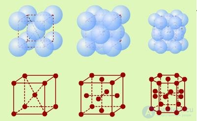
Fig. 7.1. Examples of crystal lattices

Video 7.1. Some crystallographic and physical types of crystal lattices.

Atoms undergo thermal oscillations about their equilibrium positions. If the oscillations are small, they can be regarded as harmonic. The energy of each atom consists of kinetic and potential energy. On average, each degree of freedom accounts for a kinetic energy of

and the same amount of average potential energy. Thus, the average value of the total energy per vibrational degree of freedom is equal to:

Let us now recall the classical results for the heat capacity of a crystal lattice discussed earlier. For simplicity, assume that all the atoms are identical and each has three vibrational degrees of freedom, so that it has an average energy of 3k_BT. Multiplying this quantity by Avogadro's constant N_A, we can obtain the internal energy of one mole of a crystalline solid:

where R — is the universal gas constant. Hence, for the molar heat capacity of a solid we obtain

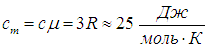
If the substance of a crystal consists of molecules having n_a atoms, then the Dulong and Petit law is modified in an obvious way:

(thus, for example, for molecules of table salt NaCl n_a = 2).

Shortcomings of the classical theory of heat capacity

1. The classical theory gives no explanation for the dependence of the heat capacity of bodies on temperature. It has been established experimentally that as absolute zero is approached, the heat capacities c_V and c_p of all bodies, including crystals, tend to zero.

2. According to the theorem of equipartition of energy, all degrees of freedom are equivalent. However, experiment leads to the conclusion that at low temperatures not all of them contribute to the heat capacity: as the temperature decreases, certain degrees of freedom become ineffective (they are said to be «frozen out»). Thus, at a temperature

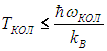
the vibrational degrees of freedom «freeze out» (here _vib — is the oscillator frequency). Quite analogously, owing to the quantization of rotational energy, the rotational degrees of freedom «freeze out»: this occurs at

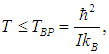
where I — is the moment of inertia of the molecule.

3. The Dulong and Petit law was formulated for any solid: metal or dielectric. However, a metal consists of positively charged ions undergoing thermal oscillations about the nodes of the crystal lattice. Between them move so-called «free» electrons, which behave like an electron gas. The presence of free electrons explains the high electrical conductivity of metals. The classical theory of heat capacity does not take into account the presence of an electron gas in metals. It accounts only for the thermal oscillations of the ions and leads to the Dulong and Petit result. Unlike dielectrics, in metals the contribution to the heat capacity made by the electrons should be taken into account. Each free electron accounts for an average kinetic energy of

Therefore, according to the classical theory, the heat capacity of the electron gas should be comparable to the heat capacity of the crystal lattice. Experiment shows that free electrons practically make no contribution to the heat capacity of metals.

7.2. Einstein's Quantum Theory of Heat Capacity

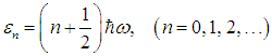
Quantum theory removed the difficulties encountered by the classical theory regarding the heat capacity of solids. Let us represent a body as a system of N oscillators that do not interact with one another. Let us apply the Boltzmann distribution law to this system, taking into account that the energy of a harmonic oscillator is quantized:

If we denote by N_n the number of oscillators with quantum number n, where

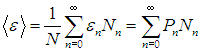
then the average energy per molecule in a state of thermodynamic equilibrium is given by

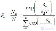
According to the Boltzmann distribution, the probability P_n of finding an oscillator in the state with quantum number n equals

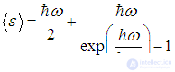
Substituting relations (7.5) and (7.3) for P_n and e_n into formula (7.4) and carrying out the summation, we arrive at the expression for the average energy of a harmonic oscillator:

Formula (7.6) differs from the expression obtained earlier by the presence of an additional first term.

This term

is the energy of the «zero-point oscillations» of the harmonic oscillator, which does not depend on temperature and therefore makes no contribution to the heat capacity of the system.

Expression (7.6) was taken by Einstein as the basis of the quantum theory of the heat capacity of solids. Einstein represented the crystal lattice of N molecules as a system of 3n_aN independent harmonic oscillators with the same natural frequency . Then the internal energy of one mole is given by the expression

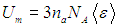
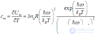
Differentiating it with respect to temperature, we obtain the molar heat capacity of the crystal lattice of solids

This is Einstein's formula for the heat capacity of crystals. At high temperatures, when

it reduces to the classical formula

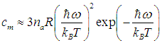
In the other limiting case of low temperatures, when

the unity in the denominator can be neglected, giving

As T, tending to 0, the resulting expression tends to zero, as required by the Nernst heat theorem (cf. Let us explain the physical meaning of this result. Because of quantum discreteness, there is a finite energy gap hw (energy gap) between the ground and excited levels of the oscillator system. The oscillator simply cannot absorb a smaller amount of energy. At zero temperature there are no excitations in the system — all the oscillators are in the ground state. With a small rise in temperature, the thermal energy is insufficient to overcome this gap, and only a small number of oscillators, proportional to

according to the Boltzmann law, go over to the first excited level. It is precisely these that are responsible for the absorption of thermal energy and, correspondingly, for the small heat capacity of the crystal at low temperatures. At high temperatures there is enough thermal energy to excite many higher-lying vibrational levels, so that the discreteness of energy no longer plays any special role — we return to the classical Dulong and Petit result.

7.3. Debye's Theory of the Heat Capacity of Solids

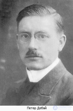
Fig. 7.2. Peter Joseph Wilhelm Debye

P. Debye (Fig. 7.2) took into account that the oscillations of atoms in a crystal lattice are not independent. The displacement of one atom from its equilibrium position entails the displacement of the atoms neighboring it. Thus, a crystal is a system of N elastically coupled atoms possessing 3N degrees of freedom. Each degree of freedom (normal mode) can be represented as a harmonic oscillator, whose average energy we have already calculated (cf. (7.6)). Because of the coupling between atoms, the frequencies of the normal modes no longer coincide with one another. The interaction of atoms causes an oscillation that arises at some point in the crystal to be transmitted from one atom to another, giving rise to an elastic wave. This wave, upon reaching the boundary of the crystal, is reflected. When the incident and reflected waves are superposed, a standing wave forms, corresponding to a normal mode of the crystal lattice. The number dN of normal modes, that is, standing waves, in the frequency interval from to + d is large, so the summation in the expression for the internal energy of the system can be replaced by integration:

Number of oscillations per unit volume. In this section we will count the number of standing waves having close frequencies . In essence, we have already carried out this calculation earlier for electromagnetic radiation, but we will repeat it here with slight modifications so that it also applies to elastic oscillations in a crystal.

Let us first consider a one-dimensional potential box of length l_x. We have already seen that a standing wave in it (whether electromagnetic, acoustic, or a de Broglie wave) is described by the function sin (kx), which must vanish at the boundaries of the box. Hence

The number n_x enumerates the various standing waves along the x, axis, and therefore the small interval of the wave vector dk_x corresponds to a number of oscillations

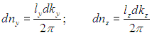
We placed the 2 in the denominator in order to avoid double counting: replacing k_x with –k_x leads to the same standing wave. In a three-dimensional box, for waves propagating along the other axes, we obtain analogous formulas

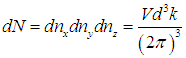
Multiplying (7.11) and (7.12), we find for the total number of standing waves in a box of volume V = l_xl_yl_z

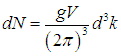
Finally, let us take into account that each standing wave may correspond to g polarizations (for de Broglie waves corresponding to particles with spin s, we have g = 2s + 1 — the number of different spin projections). Finally we obtain

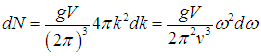
Formula (7.14) gives the number of different standing waves (differing in the number of nodes and directions of polarization) in a volume V, corresponding to a volume element d³k in wave-vector space. Next, to go over to wave frequencies, we use the relation obtained in the study of wave processes:

where v ≡ v — is the phase velocity of the wave. Hence

and finally we obtain

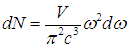
We derived formula (7.15) for a rectangular volume, but it can be shown that the shape of the volume does not affect the result. Nor does the physical nature of the oscillations whose number we counted matter much. For example, for photons v = c and g = 2 (light can have right- and left-circular polarizations). As a result we obtain the already familiar formula for the number of photon states in a volume V in the frequency interval d:

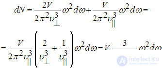
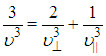
To apply (7.15) to sound waves in a crystal, let us take into account that there can be one longitudinal wave, propagating with velocity v_||, and two transverse waves with different polarizations, as with photons, propagating with velocity v_|. It is now clear how to generalize formula (7.15) to this case:

Here we have introduced the quantity v, which plays the role of a certain average between the velocities of the longitudinal and transverse waves; it is calculated from the relation

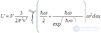
Characteristic Debye temperature. Substituting (7.17) and (7.6) into expression (7.9) for the internal energy, we obtain

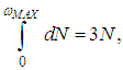
where _MAX — is the maximum frequency of the normal modes, which is determined from the relation

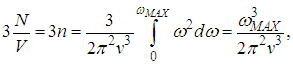
since the total number of normal modes equals the number of degrees of freedom. Using (7.17), we find

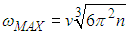
where n — is the concentration of atoms (their number per unit volume of the crystal). Thus, the maximum frequency of the normal modes, called the Debye frequency, equals

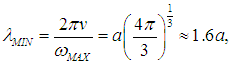
It should be noted that the shortest wavelength of an elastic wave in the crystal, which corresponds to the maximum frequency _MAX, equals

where

— the distance between neighboring atoms in the crystal lattice. This result agrees with the fact that waves whose wavelength is less than twice the interatomic distance cannot exist in the crystal.

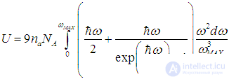
Using definition (7.22) and taking into account that for one mole of crystal the concentration of atoms is equal to

where n_a — is the number of atoms in the molecule of the crystal substance, we can write the internal energy of one mole in the form

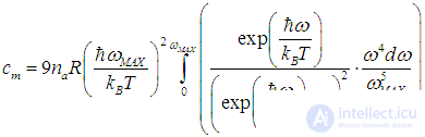
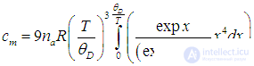
Differentiating the internal energy U with respect to temperature, we can obtain the molar heat capacity of the crystal:

Let us introduce a new parameter — the Debye characteristic temperature

and perform a change of variables in the integral (7.25)

Then the molar heat capacity of the crystal can be written in the form

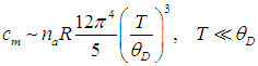
At low temperatures T << _D the upper limit of the integral will be very large, so that it can be approximately taken equal to infinity. Then the integral will represent the number

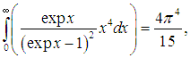
and the heat capacity turns out to be proportional to the cube of the temperature:

This approximate dependence is known as the Debye law and agrees well with experiment at sufficiently low temperatures T << _D.

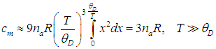
At high temperatures T >> _D the exponential in the numerator is approximately equal to unity, while the exponential in the denominator can be expanded in a Taylor series:

Then for the molar heat capacity we obtain the value

that is, the law of Dulong and Petit.

The agreement of the Debye theory with experiment can be judged from the graph in Fig. 7.3, which shows experimental points for several substances.

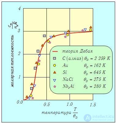
Fig. 7.3. Comparison of the Debye heat capacity theory with experimental data: substances with markedly different values of the Debye temperature and different molecular compositions are shown (n_a = 2 for NaCl and n_a = 4 for Nb₃Al), but all points lie fairly close to the theoretical curve

Example. Using the data given in the graph of Fig. 7.1, let us find the maximum vibration frequency _MAX in a gold crystal according to the Debye theory.

The Debye temperature for gold, as indicated on the graph, is _D = 162 K. Using (7.26), we find

7.4. Phonons

As within molecules, atoms in a crystal perform small oscillations about fixed equilibrium positions. Oscillations of atoms propagate through the crystal in the form of weakly interacting waves with wave vectors k and frequencies (k). Physically, normal vibrations in crystals give rise to waves of deformation of the crystal lattice (that is, elastic waves). Thus, the motion of atoms in a crystal can be described as a superposition of plane waves of various frequencies

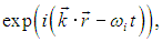
to each of which corresponds a harmonic oscillator with frequency (k).

Following de Broglie's ideas, such an elastic wave in the crystal can be associated with a quasiparticle having energy

and momentum

It is called a phonon.

Our correspondence can be represented schematically as follows (Fig. 7.4):

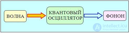
Fig. 7.4. The «wave — particle» scheme

The index i denotes the type of the corresponding wave (longitudinal, transverse, characterized by a definite dispersion law

and so on), or, as one says, a phonon mode. In the quantum-mechanical treatment, the harmonic oscillator of a given phonon mode, as we already know, can have energy

At n_i = 0 we have zero-point oscillations with energy

— there is no phonon of this mode in the solid. At n_i = 1 we have a new state with excitation energy

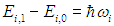
— this is precisely the phonon quasiparticle. For an arbitrary quantum number n_i the excitation energy is equal to

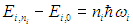
In this case we say that n_i phonons of the given mode i propagate in the solid.

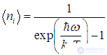
Using the results obtained above, in the case of thermodynamic (thermal) equilibrium we can find the mean number of phonons i> with frequency w_i. Indeed, we have already found the mean energy of a quantum oscillator (see (7.6), where the frequency w must now be replaced by the frequency of the elastic wave w_i). On the other hand, this same energy can be represented in the form (7.6)

Equating these expressions, we obtain

At low temperatures

the mean number of phonons decreases exponentially as T tends to 0: no excitations arise in the system. Conversely, at high temperatures

the exponential in the denominator can be expanded in a Taylor series to obtain the result

Consequently, it follows from the relation obtained that at a sufficiently high temperature an unlimited number of identical phonons can be excited simultaneously in the crystal, that is, the Pauli principle does not apply to phonons. Recall that quanta of the electromagnetic field — photons in equilibrium with the walls of a cavity — also obey this distribution.

The concept of phonons is widely used in solid-state physics. Phonons are called quasiparticles, because, although they are quite real, they exist only in crystals: outside the medium they do not exist. The idea of the existence of quasiparticles was first put forward by L.D. Landau in the 1940s.

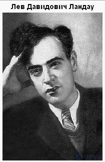
Fig. 7.5. Lev Davidovich Landau

Besides phonons there are other types of quasiparticles as well. Thermal vibrations of the lattice can be regarded as a phonon gas, which is ideal at low temperatures. At very high temperatures the lattice melts and the model of non-interacting phonons becomes inapplicable: they cease to be free. The advantage of the phonon concept is that within its framework the properties of a solid are treated as the properties of an ensemble of a large number of independent quasiparticles — an ideal phonon gas. All the notions of this model can be used to describe the behavior of the crystal lattice.

The interaction of ordinary particles (electrons, photons) with phonons can also be considered. For example, electrons exchanging phonons experience attraction. Despite the Coulomb repulsion, a bound state of a pair of electrons can even form. Such a mechanism leads to the phenomenon of superconductivity (to be discussed later).

We have already seen that the number of phonons in a solid is not constant. The more intense the thermal motion of the atoms, that is, the higher the temperature, the greater the number of phonons. As absolute zero is approached, their number tends to zero.

7.5. Indistinguishability of Identical Particles

Two particles are identical if all their physical properties coincide exactly, which excludes the possibility of experimentally distinguishing between them. In classical theory it is always assumed that we can in principle track the motion of particles and say which one flew where. Therefore, in classical theory even identical particles are in principle distinguishable. In quantum mechanics this is not so: the uncertainty principle does not allow tracking trajectories, and hence the indistinguishability of particles has a fundamental character and affects the result of calculations.

Suppose, for example, that a system of two particles is described by a Hamiltonian (energy operator)

and suppose the system is in a state with wave function

Let us introduce the operator

which interchanges the particles, that is, exchanges their position vectors:

Mathematically, the identity of the particles is expressed as the invariance (unchangeability) of the Hamiltonian with respect to the permutation operation

of these particles, which in quantum mechanics is written as the commutation condition for the operators

that is

This condition ensures the physical indistinguishability of the particles, since then the wave function will also be a solution of the Schrödinger equation with the same energy value. Indeed, if

and we act on both sides of this equation with the commutation operator

then we obtain

Because of the commutation condition, we can carry the commutation operator through the Hamiltonian:

and our equation takes the form

But we recall that commutation of operators with the Hamiltonian means conservation of their eigenvalues. Let us find the eigenvalues p of the commutation operator. For this we need to solve the equation

Taking into account the definition (7.31) of the commutation operator, we write this equation in the form

Let us again act on both sides of (7.34) with the particle permutation operator:

From (7.34) and (7.35) we obtain that

that is, p = +1. Thus, the commutation operator can have only two eigenvalues. At p = 1 the wave function is symmetric with respect to the operation of interchanging the particles:

At p = –1 we have an antisymmetric wave function:

Thus, we have obtained an important result:

A generalization of this result is valid:

Which state is realized depends on the nature of the particles under consideration.

Earlier we used these names for particles with integer and half-integer spin, respectively. In the relativistic Dirac equation, unlike the Schrödinger equation, the spin of particles arises automatically. There exists a fundamental Pauli theorem:

This theorem on the connection between spin and statistics is a consequence of the unification of quantum mechanics with the theory of relativity.

Let us turn, as an example, to the state of two atomic electrons. Neglecting the interaction between them, the wave function factors into a product of the wave functions of each electron separately:

The indices i, j denote here the complete set of quantum numbers (n, l, m, s), by which one state differs from another. Interchanging the electrons, we arrive at a state with the same energy, described by the wave function

Therefore, by virtue of the superposition principle, states described by any linear combination of these two functions are possible, all of them having the same energy. However, we now know that for electrons with spin s = 1/2 only the antisymmetric combination has physical meaning

If the states of the electrons are the same (i = j, that is, all quantum numbers coincide), then

We have again arrived at the Pauli principle:

7.6. Fermi—Dirac Statistics

Bosons and fermions have completely different statistical properties, that is, they behave differently in a collective of their own kind. Besides the direct force interaction between particles, there is a specifically quantum, exchange interaction: these are not some additional forces or fields — some particles influence the behavior of others merely by their presence. These effects are felt by particles if they are located at distances from one another that are smaller than or of the order of the de Broglie wavelength _B. At high temperatures the energies of the particles are large and _B is small — this is the domain of classical physics. At low temperatures _B increases and quantum effects dominate.

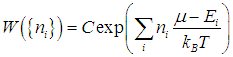
Let us consider a system of identical fermions with energies E_i in state i (where i denotes the set of quantum numbers, including spin). Let n_i denote the number of particles in state i. The basic principle of statistical physics (classical and quantum) is formulated as follows:

Here C — is the normalization constant, and — is the chemical potential. This parameter always appears when the number of particles in the system is fixed, and it equals

where the sum runs over all states. In essence, equation (7.38) is a generalization of the well-known Boltzmann distribution. It follows from the Pauli principle that n_i can take only the values 0 and 1 — in a given state i there can be either one particle or none at all.

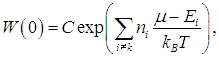
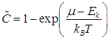
Out of the whole set of possible states of the system, let us follow some specific state k with energy E_k. With a certain probability

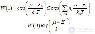
there may turn out to be no particle in it at all (n_k = 0). With probability

there will be one particle in it (n_k = 1). In writing formulas (7.39), (7.40) we used the general expression (7.38) for the probability

.

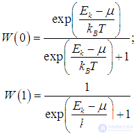
Since there is no third possibility, the condition for conservation of total probability must hold

.

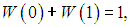whence it follows

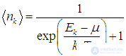
Hence, the mean number of particles

in state k turns out to be equal to

Formula (7.42) is the foundation of quantum Fermi—Dirac statistics (Fig. 7.6). At high temperatures we obtain

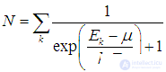
that is, a uniform distribution of particles over the states. If the number of particles N in the system is fixed, then the chemical potential m is determined from the condition

Let us also emphasize that, according to (7.42), the mean number of particles in a given state never exceeds unity. This is a direct consequence of the Pauli principle.

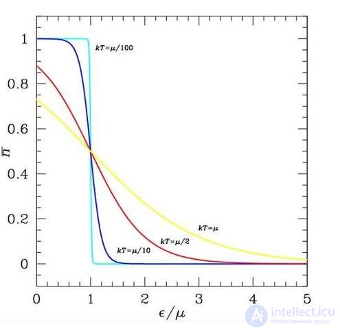
Fig. 7.6. Quantum Fermi—Dirac statistics

7.7. Bose—Einstein Statistics

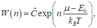
Let us now consider a system of identical bosons. In this case the number n_i of particles in state i can take any value from 0 to infinity (or from 0 to N for a fixed number of particles). Let us consider some specific state k of the system with energy E_k. Then for the probability that n particles will be found in this state, we obtain from the basic relation (7.38)

where

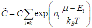
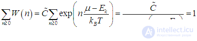
The sum W(n) over all values of n (including zero) equals the probability that in state k some number of particles will be found or none at all. Obviously, this sum must equal unity:

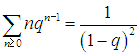
Here we used the formula

for the sum of an infinitely decreasing geometric progression at

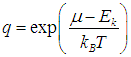
Now it is easy to find the normalization constant:

and the complete expression for the probability W(n). We are primarily interested in the mean number of particles in state k, which by the meaning of probability is expressed as

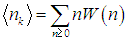
The sum of a series of the form

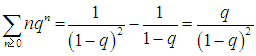
is not hard to compute by differentiating expression (7.46) with respect to q :

The left-hand side of (7.48) can be written in the form

Together with (7.48) this leads to the result:

Substituting

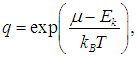
we find

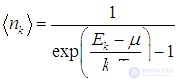
whence follows the basic relation of quantum Bose—Einstein statistics (Fig. 7.7):

The difference compared with the corresponding formula (7.42) for fermions lies only in the sign in front of unity in the denominator. Because of this, it is no longer possible to assert that the mean number of particles in a given state is always less than unity: the Pauli principle does not apply to bosons. By physical meaning, all n_k > 0, hence < E₀, where E₀ — is the minimum energy of the system (that is, the energy of the ground level). For free particles the quantity E₀ equals zero. It follows that for free bosons the chemical potential is negative. As before, there is a relation connecting and N in the case of a fixed number of particles:

At high temperatures

that is, as the temperature increases, the number of bosons in each state grows.

If the number of particles in the system is not fixed but is determined by the equilibrium conditions (for example, the equilibrium of radiation with matter, when photons are absorbed and emitted), then = 0. Applying (7.51) to a system of photons and taking into account that for photons

we arrive at formula (7.15) and its analog for phonons (7.30).

Note that at

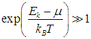
both formulas (7.42) and (7.51) reduce to the classical Boltzmann distribution. In this case

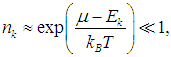
which can be interpreted as the condition of low particle density, that is, as the quantum analog of a rarefied gas: in each quantum state there is in fact no more than one particle. This means that not only is the direct interaction of the particles inessential, but so is their quantum influence on one another, the exchange effects.

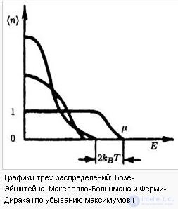
Fig. 7.7. Quantum Bose—Einstein statistics

7.8. Macroscopic Quantum Phenomena

One should not think that the laws of quantum mechanics are important only when considering phenomena on the scale of atoms and molecules. At low temperatures near absolute zero there also exist macroscopic manifestations of these laws. We shall become acquainted with them in this section.

Bose—Einstein condensation. Let us consider an ideal gas of free bosons that do not interact either with each other or with an external field. The state of a particle is specified by its momentum p and spin projection (there are altogether g = 2s + 1 possibilities, for bosons s — being an integer). The mean number of bosons in a given state k is described by formula (7.51). Since the Pauli exclusion principle does not apply to bosons, they can accumulate in one state. At zero temperature all the particles of the system must occupy the lowest energy level with E = 0. The question arises: what happens at T > 0?

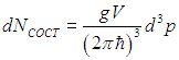
Let us again recall formula (7.14) for the number of types of vibrations, but replace the wave vector in it with the momentum of the particle:

We then obtain

By the index «st» we wish to emphasize that, dealing with quantum particles, we have started calling things by their proper names: the number of vibrations becomes in this case the number of states in which the particle can be found. The volume element of momentum space can be written in the form

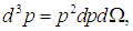
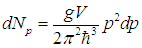
where — is the solid angle. Integrating relation (1) over the angles, we obtain the number of states dN_p, in which the magnitude of the particle's momentum lies between the values p and p + dp:

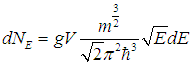
Taking into account that the energy of a free non-relativistic particle

so that

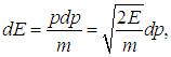
we find from (1) the number of states dN_E with energies between E and E + dE:

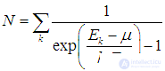
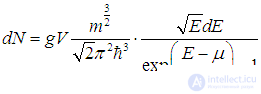
Multiplying (3) by the mean number of particles in one state, we find the number of particles falling within the same energy interval:

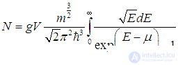
To obtain the total number of particles in the system, we integrate (4) over all values of the energy:

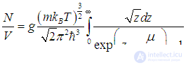
Introducing a new integration variable

we rewrite (5) in the form

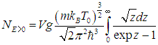
This is an equation for the chemical potential . In essence, we have rewritten formula (7.52) in a form convenient for practical application: summation over all possible states is replaced by summation (integration) over the particle's energy, while the number of states is accounted for through the use of formula (3).

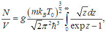
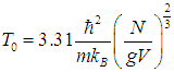
If, at a given particle concentration N/V, the temperature of the gas is lowered, then the chemical potential will increase (that is, decrease in absolute value), as follows from (6). It will reach the limiting value = 0 at a temperature T₀, defined by the equation

whence follows the expression

Let us understand the physical meaning of the combinations of parameters entering formula (8). If we denote by l the mean distance between particles, then a sphere of radius l/2 will contain one particle, that is, the particle density will be

.

Therefore, formula (8) can be rewritten in the form

.

Since the thermal energy of motion of the particles

we obtain from this

or

where _B — is the de Broglie wavelength (we have omitted inessential numerical factors in this discussion). Thus, we again arrive at the conclusion that quantum effects become noticeable when the de Broglie wavelength is of the order of the distance between particles. Formula (8) — is the general expression for the «quantum» temperature: we shall encounter it again, though only the numerical factor may change.

Thus, at T > T₀ there exists a physically admissible ( < 0) solution of equation (6). At T < T₀ the chemical potential remains equal to its limiting value 0, having nowhere further to go, and the right-hand side of the equation becomes smaller than N/V. This result is surprising, since the number of particles in the system is fixed, and the particle density, it would seem, should remain unchanged. Consequently, some fraction of these particles goes somewhere, drops out of the system, and ceases to participate in thermal motion. This means that the right-hand side of (6) at T < T₀ ( = 0) will describe those particles that do participate in thermal motion, that is, whose energy is greater than zero:

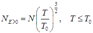
If we multiply and divide the right-hand side of (9) by

then we can single out the factor

while the remaining factor, in accordance with (7), will equal the total number N of particles in the system:

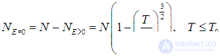
The remaining particles have zero energy; their number N_E=0 is determined as the difference N – N_E=0:

Thus, at a temperature below the critical one T < T₀ there occurs the so-called Bose — Einstein condensation — an accumulation of particles in the state with p = 0. This effect — is macroscopic, since the number of particles in the condensate is enormous, of the order of the total number of particles N. When the temperature is lowered below the critical value, the condensate appears suddenly — the system undergoes an abrupt change of properties (as is said, a phase transition occurs).

At absolute zero temperature all the particles of the system are in the condensate. As the temperature rises, some of them leave the condensate and begin to participate in thermal motion. At T > T₀ the Bose-Einstein condensate disappears: no particles remain in it. The dependence of the fraction of particles in the condensate on temperature is shown in Fig. 7.8.

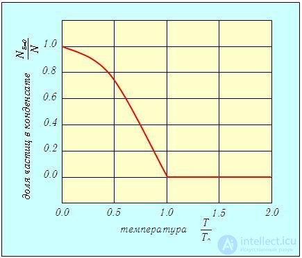
Fig. 7.8 Fraction of particles in the Bose-Einstein condensate as a function of temperature

Important to note is that condensation occurs not in ordinary space, as in the precipitation of, say, dew, but in momentum space. From the standpoint of our ordinary space, both the condensate and the normal component of the Bose gas are «mixed together», and the system remains spatially homogeneous. But there is also a similarity with ordinary saturated vapor: for example, at T < T₀ the pressure does not depend on the volume of the system, which is unusual for an ideal gas.

The phenomenon predicted by Einstein and the Indian physicist Bose many years ago was first observed experimentally in 1995 in the USA. A «gas» of 2,000 rubidium atoms, cooled almost to absolute zero (20 nK), «condensed» into a «superatom», which behaved no longer as a gas of particles, but as a single whole. Thus, a new state of matter was created that had never before existed in nature anywhere in the Universe, as was stated in the report on this work. In 2001 the authors of these experimental works were awarded the Nobel Prize.

The phenomenon of superfluidity. Superfluidity is the property of liquid helium to flow without friction through thin capillaries at low temperatures T < 2.17 K. The phenomenon was discovered by P.L. Kapitsa in 1938 (the Nobel Prize was awarded in 1978). Further studies showed that liquid helium has, as it were, two components: normal and superfluid. Owing to the absence of viscosity, superfluid helium offers no resistance to immersed bodies. In the superfluid state, liquid helium exhibits so many unusual properties that we are entitled to regard the superfluid component as a special state of matter, which is conventionally denoted He II (as opposed to ordinary He I). Let us mention only the so-called fountain effect: when the lower end of a capillary immersed in liquid helium is illuminated with a pocket flashlight, it heats up and the fraction of the superfluid component decreases. The excess pressure forces the superfluid component to flow into the capillary, which leads to the appearance of a small fountain up to 30–40 cm high. Such a flow of helium from a cold place to a hot one is unusual: in normal liquids everything happens exactly the other way around.

The phase diagram for helium is shown in Fig. 7.9.

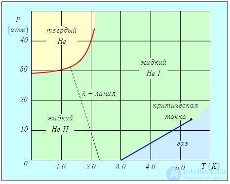
Fig. 7.9. Phase diagram for ⁴He (pressure and temperature are plotted along the axes). The dashed line shows the l-line between the normal (He I) and superfluid (He II) states

The phase transition He I => He II occurs on the so-called l-line, and the transition temperature decreases as pressure increases. The superfluid state was observed for the isotope ⁴He (superfluidity in the other isotope, ³He, was observed much later and with great difficulty, but that is another story). Since the proton and neutron that make up the helium nucleus have spin 1/2, the spin of the ⁴He nucleus — is integer, while that of ³He — is half-integer. This is where the difference between bosons and fermions arises. Particles of liquid ⁴He are bosons, and they can undergo Bose—Einstein condensation. Moreover, at a typical particle concentration in the liquid of N/V = 2·10²⁸ m^–3, a helium-nucleus mass of m = 6.7·10^{–27 kg}, and g = 1 (the total nuclear spin equals zero), formula (8) gives a Bose–Einstein condensation temperature of T₀ = 2.9 K, which is not so far from the temperature of the l-transition. It seems very tempting to connect two unusual states of matter — the Bose-Einstein condensate and the superfluid component. But everything is not as simple as it seems.

Elements of the microscopic theory of superfluidity. The point is that a liquid — is not an ideal gas: there is a strong interaction between the particles. And we considered the condensate in a system of an ideal gas of bosons. It also remains to be understood why the condensate should exhibit superfluidity. According to the microscopic theory of N.N. Bogoliubov (1947), one cannot speak of the state of individual helium atoms, but only of the state of the whole system. Here we encounter for the first time a quantum liquid — a macroscopic quantum effect. At T = 0 the system is in its ground state; as the temperature rises, thermal excitations appear — transitions to low-lying excited energy levels. Collective excitations of the atoms are quantized in a way similar to the vibrations of atoms in a crystal lattice in Debye's theory. There, quantization gave rise to phonons; here, it gives rise to — quasiparticles, individual quanta with energy . It turned out that the primary role is played by the law relating energy to momentum p — the dispersion law. In a quantum Bose-liquid, the «excitations» (quasiparticles) — are also bosons with zero spin. At low temperatures the number of quasiparticles is small, and they can be regarded as noninteracting. In this case we have an ideal gas of quasiparticles, which undergoes condensation at some critical temperature.

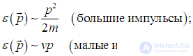
But everything, we repeat, depends on the dispersion law, the complete calculation of which is very complicated and has still not been carried out. Bogoliubov calculated the dispersion for weakly excited states. In the limiting cases his formula gives

where v — is a certain constant with the dimension of velocity. The energy in the first case is nothing other than the energy of a helium atom. The energy in the second limiting case, on the other hand, is analogous to the energy of an acoustic quantum (a phonon). The shape of the curve is shown in Fig. 7.10.

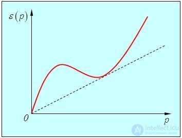
Fig. 7.10. Dependence of the quasiparticle energy in He II on their momentum (dispersion law)

Thus, for T > 0 liquid helium consists of a condensate of quasiparticles and an ideal gas of quasiparticles with energy . The helium atoms cannot be divided into «those forming the condensate» and «those giving rise to free quasiparticles»: all of them take part in forming both the ground condensate state and the ideal gas. The gas of quasiparticles can be regarded as the normal component of liquid helium, while the condensate — can be regarded as superfluid. Such a phenomenological two-component-liquid theory was developed by Landau (1941).

Superfluidity of the condensate. We have understood why an ideal gas can appear in the liquid: the free particles of the gas — are not the helium atoms themselves, but excitations of the ground state (the condensate). Now we need to understand the origin of the superfluidity of the condensate.

First, let us recall the results of classical mechanics concerning the transition to moving reference frames. Let a system K, be given, in which the position-vectors of particles with masses m_i are denoted r_i. The momentum of such a system is

and the kinetic energy

where

.

Let there also be a system K’, whose origin is given by the vector R, and let the velocity of the system K’ relative to K be

.

In the moving coordinate system, the position-vectors of the particles are

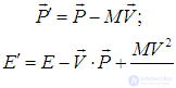
From this immediately follow the expressions for the total momentum and energy of the particles in the moving coordinate system (M — the total mass of all the particles):

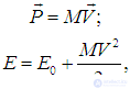
These are the nonrelativistic Galilean transformations known from classical mechanics. Following Landau's reasoning, let us now apply these formulas to an unexcited condensate flowing through a tube with velocity V. In the laboratory frame K the energy and momentum of the condensate are given by the obvious formulas

where E₀ — is the energy of the condensate at rest in the ground state. Let us take a system K’, moving with the velocity of the condensate V, so that in it the condensate is at rest. The Galilean transformations (12) then give

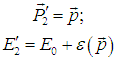
These results are obvious, and we shall only recall that all this refers to the condensate in the ground state. In the system K’ it is at rest, while past it, with velocity V the tube moves. If there is viscosity, it will show up as dissipation of energy. This cannot happen at once throughout the whole liquid: first, individual internal motions will be excited, and quasiparticles such as phonons will appear. Let an excitation arise with momentum p and energy . For the excited condensate in K’ we have quite obvious relations

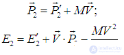
How will these formulas look in the laboratory frame? To go back to K, we use the inverse Galilean transformations:

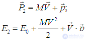
from which we find

Comparing formulas (14) and (18), we find the change in energy of the moving condensate in the laboratory frame K upon transition from the ground state to the excited state:

The formation of a quasiparticle is energetically favorable if ∆E < 0. In the most favorable case for this, the momentum p is antiparallel to the velocity V, and the change in energy of the condensate equals

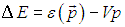
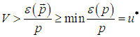
It follows that for the liquid to be decelerated, the condition must be satisfied

Here we introduced the notation u* for the parameter with the dimension of velocity — the ratio of the minimum excitation energy to the momentum. This parameter is equal to the tangent of the slope of the dashed line in Fig. 3. If the excitation spectrum is such that u*>0, as shown, then the deceleration condition is not satisfied for weak excitations: as they say, the excitation spectrum has an energy gap — a certain difference between the excitation energy and the energy of the ground state. This means that at low velocities V < u* friction is impossible. In other words, we have obtained the phenomenon of superfluidity (at small momenta the velocity u* is equal to the speed of sound). The meaning of the result obtained is that the condensate is a collective formation that responds to the loss of one of its members by an increase in energy, whereas friction should lower the energy. The dispersion law depicted in Fig. 3 is such that the condition for superfluidity is satisfied. For ordinary Bose particles with

we have

and the condition for superfluidity is not satisfied.

Conclusion: ordinary particles, even in the condensate state, do not possess superfluidity; the condensate does not form a bound collective and does not respond to the deceleration of individual particles.

Let us emphasize once again: He II — is not a mixture of different substances, and its components cannot be separated individually. It would be better to speak of the simultaneous coexistence in helium not of components, but of two types of motion — normal and superfluid.

Superconductivity.

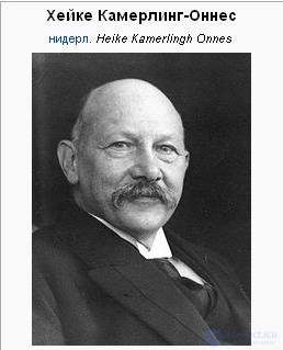
Fig. 7.11. Heike Kamerlingh Onnes

In 1911 the Dutch physicist H. Kamerlingh Onnes (Fig. 7.11) discovered a remarkable phenomenon. At a temperature of about 4 K the electrical resistance of mercury dropped abruptly to zero. The phenomenon of superconductivity was subsequently discovered by him in tin, lead, thallium, and other substances. Numerous experiments were carried out to identify the properties of the superconducting state of matter.

The most important properties of the superconducting state of matter are:

• the existence of a critical temperature T_c, at which the superconducting state arises;
• the expulsion of a weak magnetic field from the bulk of a superconductor, except for a thin layer near its surface (the Meissner effect);
• the destruction of the superconducting state upon application of a sufficiently strong magnetic field;
• the unusual temperature dependence of the heat capacity of a superconductor.

For most previously known substances the critical temperatures are of order 1–15 K. In 1986, ceramic compounds were discovered that transition to the superconducting state at temperatures of order 125 K, that is, above the boiling point of liquid nitrogen. Since superconductors had previously been obtained only by cooling the material with liquid helium, while liquid nitrogen is much cheaper to produce, the discovery of high-temperature superconductivity promises the development of numerous technical applications.

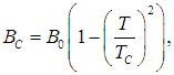
The critical value of the magnetic flux density B_c, at which the superconducting state is destroyed, depends on the temperature of the superconductor. A characteristic graph of this dependence is shown in Fig. 7.12; it is well described by the formula

where B₀ — is the critical value of the field at absolute zero temperature.

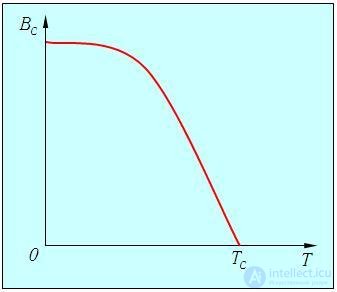
Fig. 7.12. Value of the critical magnetic field as a function of the temperature of the superconductor

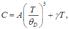
As we shall see later in our course, the heat capacity of a normal metal at low temperatures has the form

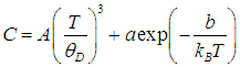
where the first term — is the already familiar contribution of the crystal lattice, described by Debye's theory, while the second term - is the contribution of the electron gas, studied in the next part of the course. In a superconductor the heat capacity at very low temperatures is determined, as experiments show, by an expression of the type

The first term has not changed: the crystal lattice is still in place as before. The dramatic change in the second term (an exponential instead of a linear function) shows that superconductivity is associated with some fundamental changes in the behavior of the conduction electrons.

The microscopic theory of superconductivity was created by J. Bardeen, L. Cooper, and J. Schrieffer, and improved by N.N. Bogoliubov. It is too complex to present in this textbook. It suffices to point out that there is a deep analogy between superfluidity and superconductivity. Owing to the interaction of electrons with phonons, an attraction arises between electrons, and under certain conditions a peculiar bound state can form — a Cooper pair of electrons with opposite spins. Such a formation is already a boson and can undergo Bose-Einstein condensation, which is precisely the prerequisite for the transition of the material into the superconducting state.

At absolute zero temperature the electron gas in a superconductor goes into a ground state possessing the properties of a condensate. What is very important, this state is separated by an energy gap E from the next, excited, state. In other words, in order to remove an electron from the ground state, it must be given some minimum energy E_g, while smaller portions of energy simply will not be absorbed. We have already seen something similar for the superfluid state, and even earlier — for heat capacity (the «freezing out» of rotational and vibrational degrees of freedom, Einstein's theory of heat capacity). The theory predicts a simple relation between the energy gap and the critical temperature:

The presence of an energy gap immediately explains the behavior of the heat capacity of the electron gas. Indeed, the energy E_g — is the minimum energy that breaks a Cooper pair, and imparting such an energy produces a pair of free electrons. Then each electron accounts for half the energy E_g/2. From statistical considerations it can be argued that the number of electrons outside the ground state is proportional to the quantity

.

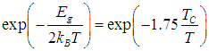The thermal energy absorbed upon excitation is proportional to

.

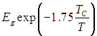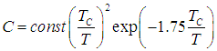
The derivative of this quantity with respect to temperature gives the heat capacity of the electron gas in the superconducting state:

At low temperatures the pre-exponential factor 1/T² changes much more slowly than the exponential, so that this law practically does not differ from the phenomenological relation (23). As the temperature changes, the value of the gap changes according to a law similar to the one shown in Fig. 4. At the critical temperature the gap disappears, and along with it the superconducting properties disappear. Note that expression (24) is analogous to the heat-capacity formula (7.8) in Einstein's theory, where a gap between the ground and excited energy levels is likewise present.

From what has been said, it is clear how important a role the energy gap plays. In a system of bosons it is responsible for the phenomena of superfluidity and superconductivity. In a system of fermions, as we shall see later, it is responsible for the difference in properties between metals, dielectrics, and semiconductors.

Studies of the phenomena of superfluidity and superconductivity have always attracted great interest from both scientists and society as a whole. The «culprit» is — the broad prospects for their practical application. They acquire particular importance in the modern world, where scientists have learned to create entirely new materials with unusual characteristics, exhibiting, for example, superconducting properties at relatively high temperatures and in sufficiently strong magnetic fields. It is no accident that more than one Nobel Prize has been awarded for research in this field, starting with Kamerlingh Onnes (the 1913 prize) and, so far, ending with the 2003 prize, awarded to A.A. Abrikosov (Russia and the USA), V.L. Ginzburg (Russia), and A.J. Leggett (the United Kingdom and the USA).