
Lecture
Это продолжение увлекательной статьи про электрическое поле в вакууме.
...
surface S is divided, that is, an integral over this surface of the form:
|
|
(1.32) |
If the vector field  is uniform, that is
  , and the surface is flat, then

Here S — is the area of this surface. To denote an integral over a closed surface, a special integral sign is used, namely one with a circle in the middle (S — a closed surface) (Fig. 1.36):

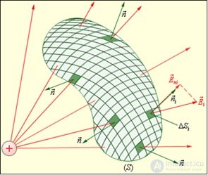
Fig. 1.36. Flux of the electric field strength vector through a closed surface
To grasp the meaning of such a quantity as the flux of a vector, it is very useful, owing to its intuitive clarity, to consider the flux of a fluid, for example, in a river or in a pipe.
Suppose, for simplicity, that an incompressible fluid with density  flows with velocity
  . Specifying the dependence of the velocity vector on the coordinates of a point and on time amounts to defining a vector field, in this case the velocity field
  . Like any vector field, the velocity field can conveniently be depicted using field lines, which in this case are called «streamlines». By definition, at any point the velocity vector of the fluid is directed tangentially to the streamline. Let us single out inside the fluid an area element
  (see Fig. 1.37) small enough that the velocity can be regarded as the same at all points of this element. Let us take a time interval
  small enough that the velocity does not manage to change appreciably during this time, and pose the following question: «What mass
  of fluid flows through the area element
  in the time
  ?». Obviously, in the given time, those fluid particles will pass through the area element that were no farther from it (along the flow) than a distance
  . Particles farther away, having the same velocity , simply will not have time to «reach» the area element in the time of interest .
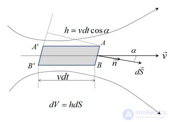
Fig. 1.37. Derivation of the relation for the flux of a vector
In the figure above, the fluid that manages, in the time  , to cross the area element
  occupies the shaded volume
  , whose magnitude, as can be seen from the figure, equals
  . Accordingly, the mass of fluid passing through the area element in the time equals
 , where
In the formula written above, the vector is precisely a characteristic of the fluid flow, determined by its density and flow velocity. The quantities and are parameters of the "experimental setup". For the same fluid flow, one can consider a different area element and choose a different time for recording the mass. The vector is called the mass flux density vector. Its unit of measurement  clearly demonstrates its physical meaning: the magnitude of the vector shows how many kilograms of fluid flow per second through a square meter of area element perpendicular to the flow. Its projections onto the axes have the same meaning, with the difference that
  is numerically equal to the mass of fluid flowing per second through a square meter of an area element perpendicular to the OX axis,
  – … the OY axis, and so on.
If is divided by the density  , the result is
  — the volume flux density vector, measured in
  . The magnitude of this vector is numerically equal to the number of cubic meters of fluid passing per second through a square meter of area element perpendicular to the fluid flow. Knowledge of this vector is required, for example, in calculating the throughput capacity of a gas or oil pipeline, as well as of a water pipeline.
Gauss's theorem for the vector  , proved below (see relation ), shows that the sources of an electrostatic field are electric charges.
Let us first consider a particular, but very simple, example of a direct calculation of the flux of a vector through a surface.
Example 6. A hemisphere of radius R with a flat base is placed in a constant uniform electric field E, perpendicular to the base of the hemisphere (Fig. 1.38). Find the flux of the field strength vector through the base of the hemisphere, through the hemisphere itself, and through the entire closed surface of this body.
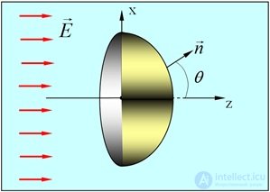
Fig. 1.38. Example of calculating the flux of the electric field strength vector
Solution. The simplest thing is to calculate the flux  through the base of the hemisphere. Let us direct the z axis along the field. The direction of the outward normal vector to the base is opposite to the direction of vector E. At the same time, vector E is the same at all points of the base. The flux through the base turns out to be equal, with the opposite sign, to the product of E and the area of the base
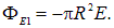
Let us now find the flux of the field strength through the surface of the hemisphere. Using spherical coordinates — the angles  and
and  — to determine the position of a point on the hemisphere, we see that

and

Therefore, the flux through an elementary area element on the hemisphere equals

Taking into account that

and
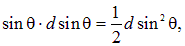
we write the flux in the form
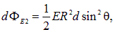
from which we find the total flux through the surface of the hemisphere

We have found that the flux through the surface of the hemisphere is equal in absolute value to the flux through its base, so that, taking signs into account, the total flux through the closed surface equals zero
 .
.
Gauss's theorem for the vector  makes it possible to relate the flux of the field strength vector through a certain closed surface to the magnitude of the charges located inside this surface. Let us first consider a particular case, namely: let us determine the flux of the field strength vector through an arbitrary imaginary spherical surface, at the center of which a point charge is located.
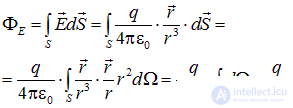
The field lines of the vector field  of a point charge are radial straight lines, directed away from the charge if it is positive, and toward the charge if it is negative (see Fig. 1.12). The flux of the field strength vector of a point charge through a spherical surface of radius r, whose center coincides with the position of the charge and the origin of coordinates, equals
|
|
(1.33) |
Here  , where
  — is an element of solid angle, we made use of the value of the total solid angle

It can be shown that the flux of the field strength vector through any closed surface enclosing a charge q does not depend on the shape of the surface and equals  , just as for a sphere. The physical meaning of this statement, again, is that field lines begin and end on charges. Therefore, a continuous (unbroken) deformation of the surface (shown by a dotted line in Fig. 1.39-1) will not change the total number of field lines emerging outward. As a consequence, the flux through an arbitrary surface enclosing the charge will be the same as for a sphere (see Fig. 1.39-1).
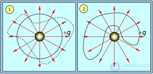
Fig. 1.39. Flux of vector E through a closed surface:
1 — the charge is inside the surface; 2 — the charge is outside the surface
If, however, the charge is located outside the space bounded by the closed surface, then the field lines pierce the surface an even number of times (from outside in and from inside out), so that the total flux through a surface not enclosing the charge equals zero (Fig. 1.39-2).
The derivation of Gauss's theorem for a point charge located at an arbitrary point is given in Supplement 5.
Suppose now that inside and outside a given closed surface there is an arbitrary number of point charges of any sign. By virtue of the superposition principle, the total field strength will be a vector sum of the field strengths of each of the charges

The total flux of the field strength through this surface is
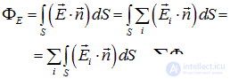
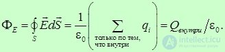
Using , we obtain the relation known as Gauss's theorem for the vector  :
:
|
The flux of the electric field strength vector through a closed surface equals the total charge inside this surface divided by
|
Let us stress once again a trivial but important circumstance: if there are no charges inside the surface, then the flux of vector  through this surface equals zero (Fig. 1.40). The sources of an electrostatic field are electric charges, and the total power of the sources of the electrostatic field inside the surface equals
  . The presence in the last formula of the electric constant
  is a result of the choice of the system of units (SI) and has no physical meaning.
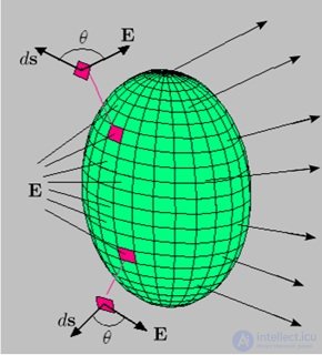
Fig. 1.40. If there are no charges inside the surface, then the flux of vector  through this surface equals zero
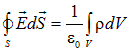
For a continuous distribution of charge over a volume, it is natural to write Gauss's theorem in the following form
|
|
(1.35) |
On the right-hand side of this relation, the integral is taken over the volume  bounded by the surface
  , the flux
  through which is computed on its left-hand side. For a continuous distribution of charge over some surface, an integral of the form
  will stand on the right, but only over that part
  of the charge-bearing surface which turns out to be inside the surface
  standing on the left. For a continuous distribution of charge along some line
  , an integral of the form
  will stand on the right, likewise only over that part
  of the charge-bearing line which turns out to be inside the surface . In short, it is necessary, by any acceptable means, to compute the charge inside the closed surface over which the flux of the electric field strength vector is being computed.
Examples of field calculations, in which the main tool is Gauss's theorem, are given in the following section 1.5.
Gauss's theorem for the vector 
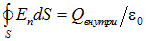
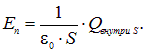
can be successfully used as an effective tool for calculating the field strength and potential of the electric field of a given charge distribution, when the integral standing on the left can be turned into the product of the area of the surface over which the integration is performed and the magnitude of the component  of vector normal to the surface, that is, when
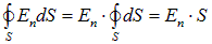 .
.
It is quite obvious that for calculating the vector this will be sufficient, firstly, when the vector is perpendicular to the surface. Consequently, the surface of integration must be an equipotential surface of the field being calculated. Its shape must be known in advance. Finally, secondly, at all points of this — equipotential — surface, the component normal to it must have the same magnitude, otherwise it cannot be taken outside the integral sign, and it will only be possible to find the value of  averaged over the equipotential surface. Let us stress that from the fact that the surface is equipotential, namely, from the fact that
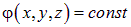
it by no means follows that also

at the points of this surface. Getting ahead of ourselves, let us point out that, for example, the surface of a charged conductor, given equilibrium distribution of charge on it, is always equipotential, but if it is not a sphere but a body of complex shape, then in the vicinity of protrusions (points) the field strength can be orders of magnitude greater than in the vicinity of hollows on the surface. The requirement of constancy of  is a separate requirement.
From what has been said above it follows that Gauss's theorem is able to lead quickly and simply to a result (the vector  ) only in the case where the charge distribution creating the field possesses a high degree of symmetry, so that, correspondingly, the shape of the equipotential surfaces of the field is known in advance and there is confidence that
  on these surfaces. If all this holds, then the solution looks as simply as follows:
|
|
(1.36) |
 according to the symmetry of the charge distribution and to compute the charge inside .
Spherical symmetry
For a spherically symmetric charge distribution, the field it creates is likewise spherically symmetric. Vector (and scalar) fields with such symmetry are also usually called central fields. A centrally symmetric field can in the general case be written in the form
 .
.
Here  — is the radius vector, starting at the center of symmetry of the field, r — its magnitude,
  — the radial component of the field strength, depending only on the distance
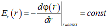
  to its center of symmetry. The potential of such a field depends only on and
|
|
(1.37) |
And, moreover, as follows from , with an arbitrary normalization the potential of the field has the form
|
|
(1.38) |
Thus, the conditions of applicability are satisfied and we can make use of this relation.
Let us take as  an equipotential spherical surface of some running radius r, its area
  . In view of the assumed continuity of the charge distribution, for
  we use the expression:
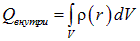 .
.
where  — is the volume charge density. Again, taking into account the spherical symmetry of the charge distribution —
  depends only on , it is natural to take as the volume element
  an infinitesimally thin spherical shell with inner radius
  and outer radius
  . The volume of such a shell is
  , as a result we obtain
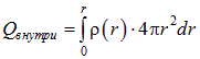 .
.
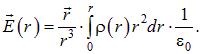
Finally, for any spherically symmetric charge distribution, when  , we obtain
|
|
(1.39) |
To continue the calculation requires specifying the form of the dependence of the charge density  on the magnitude of the radius vector
  .
.
The field uniform over the volume of a charged sphere
A distribution of charge, uniform over the volume of a sphere of radius  , with total charge
  (Fig. 1.41) means that its charge density
  has the form
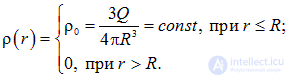
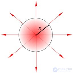
Fig. 1.41. Field lines of the electric field of a uniformly charged sphere
One should not forget that, by the condition, there are no charges outside the sphere.
Since at the point  the charge density changes abruptly: the limit «from the left» is nonzero
  , while the limit «from the right» equals zero
 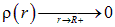 , the calculation will have to be carried out in two stages: first for a spherical surface of radius
  (it lies inside the sphere), and then for a spherical surface of radius
  (it encloses the sphere). In the first case
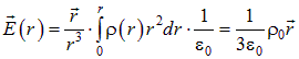
 .
.
Correspondingly, the field
|
|
(1.40) |
grows linearly with increasing distance from the center of the sphere, which is explained simply: the surface area is  , and the charge inside it is
In the second case the integral is «cut off from above» at  :
:

and the field
 .
.
In the last expression it is taken into account that  , where
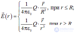
  — is the total charge of the sphere. Thus, outside the sphere its field is the field of a point charge equal to the total charge of the sphere and placed at the center of this sphere:
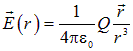 .
.
Both expressions can be combined into a single formula. If we use the total charge of the sphere  , we get:
|
|
(1.41) |
If instead of the total charge of the sphere  we use the charge density
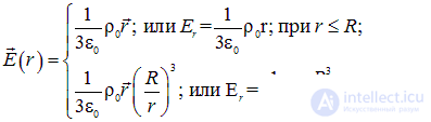
  as the parameter, these formulas take the following form (Fig. 1.42):
|
|
(1.42) |
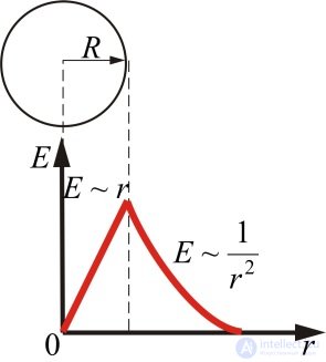
Fig. 1.42. Distribution of the electric field strength of a uniformly charged sphere
The formulas express one and the same dependence, their convenience is determined by which parameters are given:  or
or  . From these formulas it is evident that at the surface of the sphere
  the field strength is continuous, that is, it has no discontinuity. This is due to the fact that in this case the discontinuity of the charge density at the surface of the sphere is of the first kind — of finite magnitude: from
  to zero. Therefore, both in and in , non-strict inequality signs are placed in the upper and lower formulas. In what cases the field strength can undergo a discontinuity will become clear from the following example.
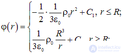
The potential of the field is easily found by substituting, for example,  from into and carrying out the integration. We obtain:
|
|
(1.43) |
where  and
and  — are constants of integration, which are found from the following considerations. The constant is determined from the normalization condition, for example, to zero at infinity
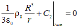
From which  . The constant
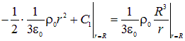
  is determined from the condition of continuity of the potential at the surface of the sphere, that is, at
  :
:
|
|
(1.44) |
or
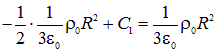
from which
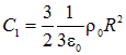
Note that the requirement of continuity of the potential is often called «matching» of two solutions at the interface. In this case it is the interface between two regions: the region where there is charge (inside the sphere), and the region where there is none (outside the sphere). Already at this point it can be noted that the potential is continuous in all cases except one: the so-called «double layer». Imagine a surface, on one side of which a positive charge is distributed with density  , and on the other side of which a negative charge is distributed with density
  . Such a surface is called a double layer; on this surface the potential undergoes a discontinuity. Such a (flat) surface can be obtained by bringing the two plates of a parallel-plate capacitor arbitrarily close together. The same thing can be done for a capacitor of any shape, for example, spherical or cylindrical. In all other cases the potential is continuous.
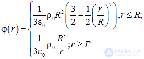
Substituting the obtained values of the integration constants into , we write the final result in the form
|
|
(1.45) |
With such a normalization, the potential at the center of the sphere is nonzero and equals
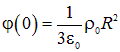 .
.
The results obtained are illustrated by Figure 1.43 below.
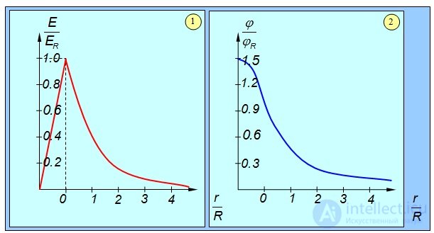
Fig. 1.43. Field strength (1) and potential (2) of the electric field of a uniformly charged sphere of radius R, in units of the field strength and potential at its surface (r = R)
The field of a uniformly charged spherical surface
In this case of a uniform distribution of charge over a spherical surface, as in the previous case, spherical symmetry holds, so the general formulas obtained above are applicable here as well. However, one must treat them with a certain caution for the following reason. The volume charge density entering the right-hand side behaves in this case in the following interesting way:
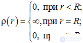
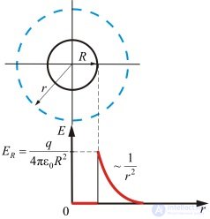
Fig. 1.44. Field strength of a uniformly charged sphere
Indeed, charge is present only on the surface, that is at  , everywhere inside, that is at
  , and everywhere outside, that is at
  , there are no charges. The fact that the volume charge density
  at points of the surface
  goes to infinity (+∞ in the case of positive charge and –∞ in the case of negative charge) can be shown as follows. In the figure alongside, a portion of some surface is depicted, over which charge is distributed with surface density
  . To determine the magnitude of the volume charge density at some point of the surface, consider a cylinder (Fig. 1.45), whose upper base is above the surface and whose lower base is below the surface. The area of the bases of the cylinder equals
  , the height —
  , the volume
  . The charge inside the cylinder is
  , the volume charge density is by definition equal to the limit of the ratio of the charge located inside some volume to the magnitude of that volume as the latter tends to zero (with all the reservations regarding a «physically infinitesimal» volume). We obtain
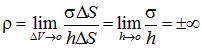
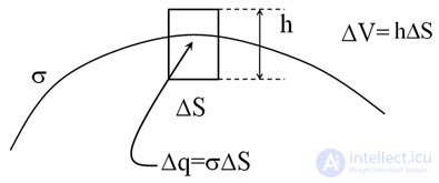
Fig. 1.45. Charge density on the surface
It is important that the density on the surface equals infinity. Functions of this kind (everywhere zero, except at one single point — where it is infinite) belong to the class of so-called generalized functions, called Dirac functions in honor of the physicist Dirac, who first introduced such a function into physics to meet the needs of quantum mechanics. We will not here examine such functions in detail or use them in calculations. Our goal is to show that considering formally infinitesimally thin charged surfaces leads to the appearance of (infinite) discontinuities in the volume charge density, which, in turn, gives rise to infinite discontinuities in the electric field strength at such a charged surface. Let us stress that the potential of the field remains continuous in this case.
The way out of this situation is simple. For all  we use the first of the formulas with
  , and obtain that everywhere inside a uniformly charged spherical shell there is no field:
  . For all
  the second formula from is valid. As in the case of a sphere uniformly charged over its volume, outside a uniformly charged spherical shell, its field is the field of a point charge placed at the center of this shell and equal to its total charge. In this case, of course,
  .
.
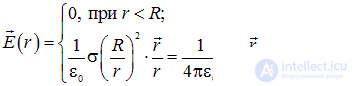
The final result is as follows:
|
|
(1.46) |
On the spherical surface itself, the field strength in this case undergoes a discontinuity. The dependence of the radial component of the field on the distance to the center of the spherical surface is shown in Fig. 1.46.
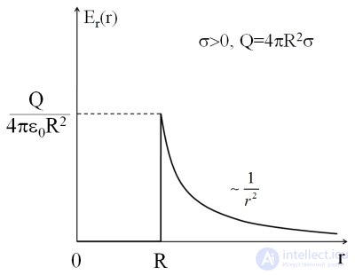
Fig. 1.46. Dependence of the field on the distance to the center of the spherical shell
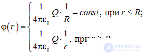
The dependence of the potential on the distance to the center of the spherical shell can be obtained by integrating . With normalization to zero at infinity, the result looks as follows:
|
|
(1.47) |
The dependence is shown in Fig. 1.47.
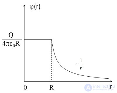
Fig. 1.47. Potential of a uniformly charged sphere
A uniform (homogeneous) distribution of charge over an infinitely long cylindrical surface (Fig. 1.48) possesses cylindrical, translational, and mirror symmetry. This means the following. Upon rotation of such a charge distribution around the axis of the cylindrical surface through any angle, it coincides with itself. Upon a shift (translation) of such a charge distribution by any distance along the axis of symmetry, it likewise coincides with itself. And, finally, if through any point on the axis of symmetry a plane perpendicular to the axis is drawn, and the «upper» part of the charge distribution is reflected in this plane as in a mirror, then the reflection of the «upper» part will coincide with the «lower» part, and conversely, the reflection of the «lower» part will coincide with the «upper» part. In other words, this charge distribution is invariant with respect to the indicated transformations. Consequently, the electric field created by this charge distribution must also be invariant (coincide with itself) under the indicated transformations.
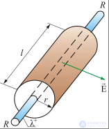
Fig. 1.48. Infinitely long cylindrical surface
Let us introduce a cylindrical coordinate system: let the axis  be directed along the axis of symmetry,
  — the distance to the axis of symmetry,
  — the azimuthal angle, the angle of rotation around the axis of symmetry,
  — as before, the potential of the field.
From the symmetry properties it follows that the potential of the field cannot depend either on the coordinate  — the translational symmetry would be violated, or on the coordinate
  — the axial (cylindrical) symmetry would be violated. There remains only the dependence on
  — the distance to the axis of the cylinder. Thus:
|
|
(1.48) |
Correspondingly
|
|
(1.49) |
the electric field strength vector is directed along radial straight lines perpendicular to the axis of symmetry (Fig. 1.49), and its magnitude depends only on the distance to the axis. The equipotential surfaces are cylinders coaxial with the charged cylindrical surface.
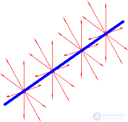
Fig. 1.49. The electric field strength vector is directed along radial straight lines
Using these circumstances, let us integrate, on the left-hand side of Gauss's theorem, over the closed surface  of a cylinder with base radius
  and height
  , coaxial with the charged cylindrical surface of radius
  under consideration. The flux through the bases of the cylinder equals zero, since on the bases
  , while the flux through its lateral surface equals the product of
  and its area:
  . Correspondingly, the total flux (through the entire closed surface of the cylinder under consideration) of the vector
  equals
|
|
(1.50) |
At  , the charge located inside the cylinder equals
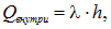
where  — is the linear charge density, numerically equal to the charge per unit length of the cylindrical surface. According to Gauss's theorem
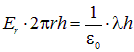
from which for  we obtain
 .
.
At  , inside the cylinder, through the surface of which the flux of vector
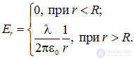
  is calculated, there are no charges, and therefore the field equals zero. Combining these two results, we finally obtain (Fig. 1.50):
|
|
(1.51) |
Owing to the surface character of the charge distribution (see the previous calculation for more detail), on the charged surface itself, that is, at  , the radial component of the field
  undergoes a discontinuity.
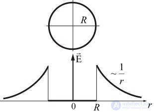
Fig. 1.50. Electric field strength of a uniformly charged cylindrical surface
Integration of (1.51) (see also (1.49)), the
продолжение следует...
Часть 1 1. The electric field in vacuum
Часть 2 1.4. Flux of a vector. The Ostrogradsky–Gauss theorem for a
Часть 3 1.5. Application of Gauss's theorem for calculating the electric field
Часть 4 Appendices - 1. The electric field in vacuum
Часть 5 - 1. The electric field in vacuum







Comments