
Lecture
Even in ancient times it was known that certain minerals, for example magnetite (chemical composition 31% — Fe, 69% — O), are capable of attracting one another, as well as attracting pieces of iron. Such bodies are called magnets. The greatest force of attraction is possessed by the opposite ends of a magnet, which are called magnetic poles (Fig. 6.1).
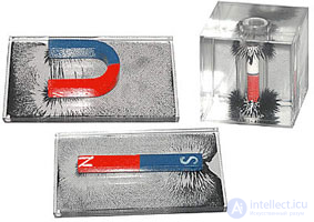
Fig. 6.1. Permanent magnets of various shapes
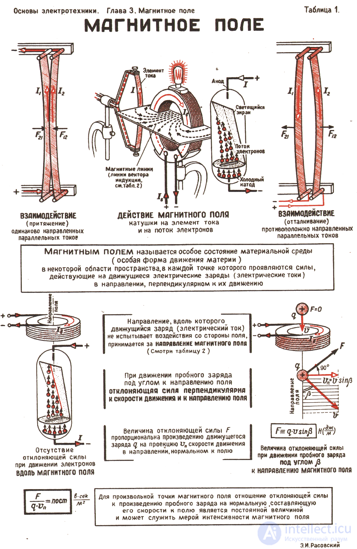
Earlier we considered a current loop and associated with it, characterizing its properties, the magnetic moment vector  , where
  — is the normal to the plane of the loop, whose direction is given by the right-hand screw rule (Fig. 6.2). The torque
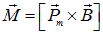
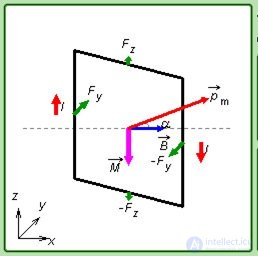
Fig. 6.2. A current loop in an external magnetic field
tends to rotate the loop. To increase the angle  between the magnetic moment of the loop and the direction of the magnetic induction of the field, work must be done

which increases the potential energy of the loop dP = –dA. Hence
|
|
(6.1) |
The energy reaches its minimum when the magnetic moment of the loop becomes parallel to the magnetic induction vector of the field ( ); the antiparallel position (
 ) corresponds to an unstable equilibrium position. All this means that a current loop behaves like a magnetic needle (a magnetic dipole). Moreover, a current loop cannot be divided into two independent poles — north and south. We have arrived at Ampère's hypothesis: all magnetic phenomena are ultimately generated by elementary currents flowing in the structural units of matter.
The following experiments serve as illustrations of the analogous behavior of a magnetic needle (magnet) and a current in a wire:
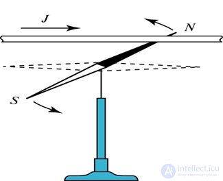
Fig. 6.3. Rotation of a magnetic needle
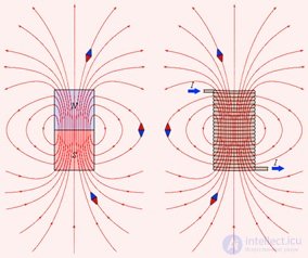
Fig. 6.4. Magnetic needles orient themselves along tangents to
the field lines of the magnetic field of a permanent magnet and a solenoid
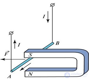
Fig. 6.5. Action on a current-carrying wire
A magnetic needle is not only a device that registers an external magnetic field — it is itself a small magnet, creating its own field. This means that a current loop must also create its own magnetic field, similar to the field of the needle. Consequently, any electric current in a conductor creates a magnetic field around it. In particular, such a field must be created by a moving electric charge.
Now let us try to guess what magnetic field is produced by a charge q moving with velocity v (Fig. 6.6). Our starting point will be the analogy between electric and magnetic phenomena. Let us recall what we already know. To obtain the force acting on a charge in an electrostatic field, we multiply the magnitude of the charge by the field strength vector

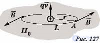
Fig. 6.6. The magnetic field of a moving charge
To obtain the Lorentz force exerted by the magnetic field on a moving charge, we also perform a multiplication operation: we take the vector (cross) product of  with the magnetic induction
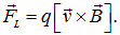
Let us apply the same technique to guess the magnetic field of a moving charge.
The electric field of a stationary point charge equals
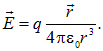
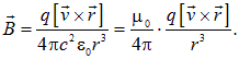
Let us replace q with the vector , the electric field with the magnetic field, and the operation of ordinary multiplication with vector multiplication. We obtain
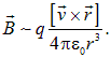
We have not placed an equals sign here, since the dimensions on the left- and right-hand sides of the equation do not quite match. From the expression for the Lorentz force it follows that the dimension of magnetic induction equals
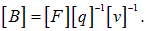
The dimension of the right-hand side of the equation, however, equals

For the dimensions of both sides to match, the right-hand side must be divided by the square of some velocity. The velocity of the particle has already been used, and the only remaining possibility is the fundamental physical constant, the speed of light c
|
|
(6.2) |
We have introduced here a new constant  , related to
  by the relation
|
|
(6.3) |
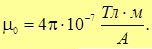
It is called the magnetic constant; its numerical value turns out to be equal to
|
|
(6.4) |
Of course, expression (6.2) has been obtained only by analogy and cannot be regarded as strictly derived. However, let us see what consequences it leads to.
Let us take an element of the conductor  , carrying a current I (Fig. 6.7). The direction of the vector I
  , called the current element, coincides with the direction of the current in the conductor, that is, with the direction of the vector
  of the drift velocity of the positive charges.
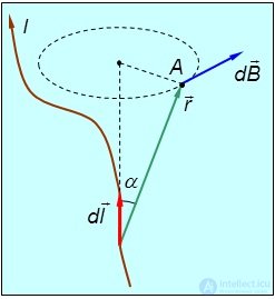
Fig. 6.7. The magnetic field created by a current element
The total charge of the current carriers in this element equals dq = enSdl, where e — is the charge of the carriers, n — is their concentration, and S — is the cross-sectional area of the conductor. Let us substitute this charge into expression (6.2) and obtain (Fig. 6.8)
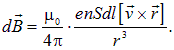
The current strength is given by the expression

whence, taking into account that

we obtain
|
|
(6.5) |
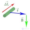
Fig. 6.8. The direction of the magnetic induction vector
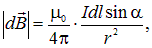
The vector  is drawn from the current element to the observation point A. Accordingly, the modulus of the vector
  equals
|
|
(6.6) |
where  — is the angle between the direction of the given current element
  in 1820 by Biot (Fig. 6.9) and Savart (Fig. 6.10) and formulated by Laplace (Fig. 6.11)
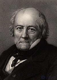
Fig. 6.9. J. Biot (1774–1862) — French physicist, geodesist, and astronomer
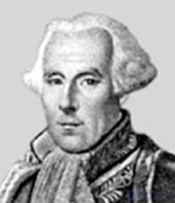
Fig. 6.10. F. Savart (1791–1841) — French physicist
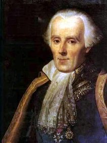
Fig. 6.11. P. Laplace (1749–1827) — French mathematician, physicist, and astronomer
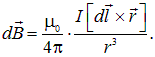
The Biot — Savart — Laplace law determines the magnetic induction  at any point of the magnetic field created by a constant electric current flowing through a conductor of any shape (see Fig. 6.7). To do this, relation (6.5) must be integrated along the entire conductor. Here the magnetic inductions from different current elements are added vectorially, that is, the superposition principle is used for magnetic fields.
Let us calculate the field created by a current flowing through a thin straight wire of infinite length.
The magnetic induction at an arbitrary point A (Fig. 6.12), created by the conductor element dl, will equal
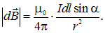
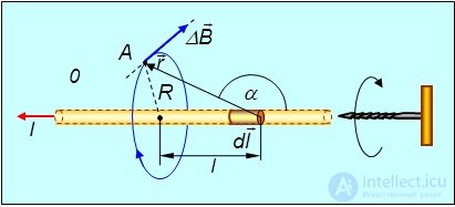
Fig. 6.12. The magnetic field of a straight conductor
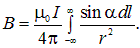
The fields from different elements have the same direction (tangent to a circle of radius R lying in a plane orthogonal to the conductor). This means we can add (integrate) the absolute values 
|
|
(6.7) |
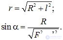
Let us express r and sin through the integration variable l
|
|
(6.8) |
Then (6.7) can be rewritten as
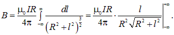
Thus,
|
|
(6.9) |
The pattern of the magnetic field lines of an infinitely long straight current-carrying conductor is shown in Fig. 6.13.
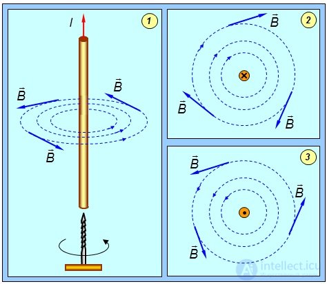
Fig. 6.13. Magnetic field lines of a straight current-carrying conductor:
1 — side view; 2, 3 — cross-section of the conductor by a plane perpendicular to the conductor
To denote the direction of the current in a conductor perpendicular to the plane of the figure, we shall use the following notations (Fig. 6.14):
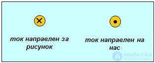
Fig. 6.14. Notations for the direction of the current in a conductor
To denote the direction of the current in a conductor perpendicular to the plane of the figure, we shall use the following notations (Fig. 6.14):
Let us recall the expression for the electric field strength of a thin filament charged with linear charge density 

The similarity of the expressions is obvious: we have the same dependence on the distance to the filament (current), and the linear charge density has been replaced by the current strength. But the directions of the fields differ. For the filament, the electric field is directed radially. The field lines of the magnetic field of an infinite straight current-carrying conductor form a system of concentric circles enclosing the conductor. The directions of the field lines form a right-handed screw system with the direction of the current.
Fig. 6.15 shows an experiment studying the distribution of the magnetic field lines around a straight current-carrying conductor. A thick copper conductor is passed through holes in a transparent plate onto which iron filings have been sprinkled. After a constant current of 25 A is switched on and the plate is tapped, the filings form chains repeating the shape of the magnetic field lines.
Around a straight wire perpendicular to the plate, ring-shaped field lines are observed, most densely arranged near the wire. As the distance from it increases, the field decreases.
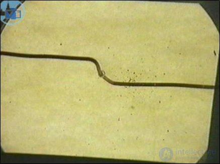
Fig. 6.15. Visualization of the magnetic field lines around a straight conductor
Fig. 6.16 shows experiments studying the distribution of the magnetic field lines around wires passing through a cardboard plate. Iron filings sprinkled on the plate line up along the magnetic field lines.
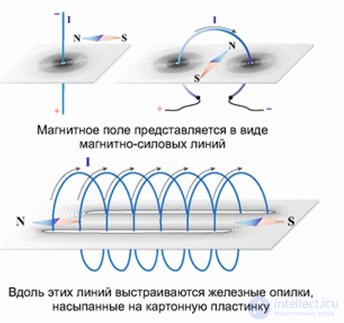
Fig. 6.16. Distribution of the magnetic field lines
near the intersection of the plate with one, two, and several wires
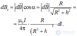
The magnetic field strength on the axis of a circular current (Fig. 6.17-1), created by a conductor element Idl, equals
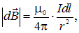
since in this case

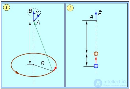
Fig. 6.17. The magnetic field on the axis of a circular current (left) and the electric field on the axis of a dipole (right)
When integrating around the loop, the vector  will trace out a cone, so that in the end only the component of the field along the 0z axis «survives». It is therefore sufficient to sum the quantity
|
|
(6.10) |
The integration

is carried out taking into account that the integrand does not depend on the variable l, and that

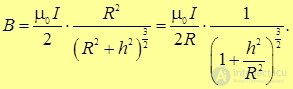
Accordingly, the total magnetic induction on the axis of the loop equals
|
|
(6.11) |
In particular, at the center of the loop (h = 0) the field equals
|
|
(6.12) |
At a large distance from the loop (h >> R) the unity under the radical in the denominator can be neglected. As a result we obtain
|
|
(6.13) |
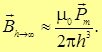
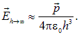
Here we used the expression for the modulus of the magnetic moment of the loop Pm , equal to the product of I and the area of the loop  The magnetic field forms a right-handed screw system with the circular current, so that (6.13) can be written in vector form
|
|
(6.14) |
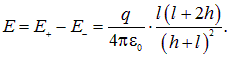
For comparison, let us calculate the field of an electric dipole (Fig. 6.17-2). The electric fields from the positive and negative charges are, respectively,
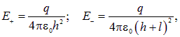
so that the resulting field will be
|
|
(6.15) |
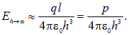
At large distances (h >> l) we hence obtain
|
|
(6.16) |
Here we used the concept, introduced in (3.5), of the electric dipole moment vector  . The field E is parallel to the dipole moment vector, so that (6.16) can be written in vector form
|
|
(6.17) |
The analogy with (6.14) is obvious.
The field lines of the magnetic field of a circular current loop are shown in Fig. 6.18. and 6.19
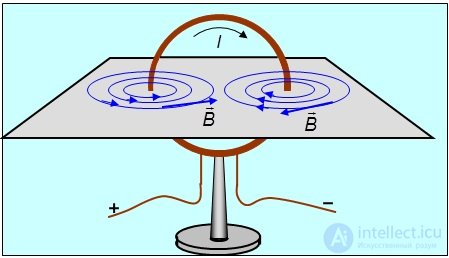
Fig. 6.18. Field lines of the magnetic field of a circular current loop at small distances from the wire
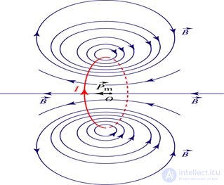
Fig. 6.19. Distribution of the magnetic field lines of a circular current loop in the plane of its axis of symmetry.
The magnetic moment of the loop is directed along this axis
Fig. 6.20 shows an experiment studying the distribution of the magnetic field lines around a circular current loop. A thick copper conductor is passed through holes in a transparent plate onto which iron filings have been sprinkled. After a constant current of 25 A is switched on and the plate is tapped, the filings form chains repeating the shape of the magnetic field lines.
The magnetic field lines for a loop whose axis lies in the plane of the plate become denser inside the loop. Near the wires they have a ring shape, and far from the loop the field falls off rapidly, so that the filings are practically not oriented.
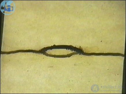
Fig. 6.20. Visualization of the magnetic field lines around a circular current loop
Example 1. An electron in a hydrogen atom moves around a proton in a circle of radius aB = 53 pm (this quantity is called the Bohr radius, after one of the creators of quantum mechanics, who was the first to calculate the orbital radius theoretically) (Fig. 6.21). Find the strength of the equivalent circular current and the magnetic induction B of the field at the center of the circle.
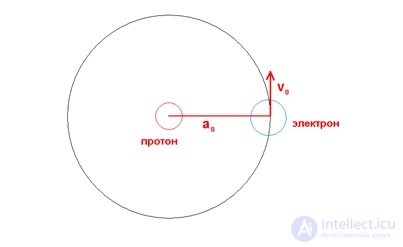
Fig. 6.21. An electron in a hydrogen atom
Solution. The charges of the electron and the proton are equal in magnitude (e) and opposite in sign. The electron is acted upon by the Coulomb attraction force of the proton, which creates a centripetal acceleration
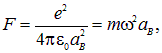
whence we find the angular velocity of the electron's motion along the circular orbit
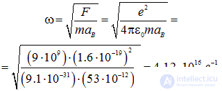
The period of revolution of the electron around the nucleus equals
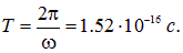
If we imagine an imaginary area orthogonal to the electron's trajectory, then during the time T a charge e passes through it. Therefore the equivalent current strength equals

The electron's velocity equals v =  aB = 2.18·106 m/s. The moving charge creates a magnetic field at the center of the orbit

The same result can be obtained using expression (6.12) for the field at the center of a current loop, the strength of which we found above

Example 2. An infinitely long thin current-carrying conductor with a current of 50 A has a ring-shaped loop of radius 10 cm (Fig. 6.22). Find the magnetic induction at the center of the loop.
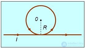
Fig. 6.22. The magnetic field of a long conductor with a circular loop
Solution. The magnetic field at the center of the loop is created by the infinitely long straight wire and the circular loop. The field from the straight wire is directed orthogonally to the plane of the figure, «toward us», and its magnitude equals (see (6.9))

The field created by the ring-shaped part of the conductor has the same direction and equals (see 6.12)

The total field at the center of the loop will equal
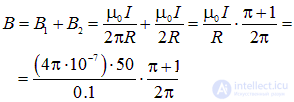
|
A solenoid is a cylindrical coil consisting of a large number of turns of wire forming a helical line (Fig. 6.23-1). |
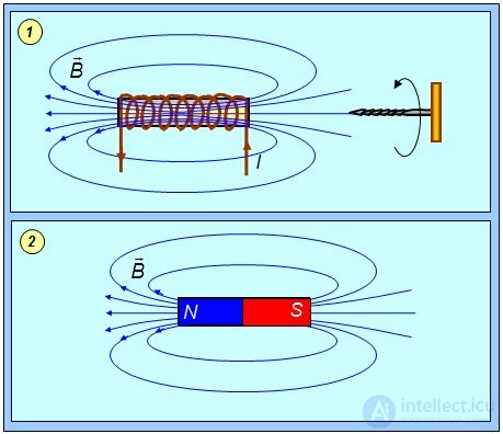
Fig. 6.23. Magnetic field lines: 1 — of a solenoid; 2 — of a bar magnet
The magnetic field of a solenoid resembles the field of a bar magnet (Fig. 6.23-2).
If the turns are wound tightly together, the solenoid is a system of circular currents having a common axis.
If the solenoid is considered sufficiently long, the magnetic field inside the solenoid is uniform and directed parallel to the axis. Outside the solenoid, far from the ends, the magnetic field must also have a direction parallel to the axis, and at a large distance from the solenoid it must be very weak. The field decreases according to the law

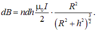
Let us calculate the field inside the solenoid. Let us take an element of the solenoid of length dh, located at a distance h from the observation point. If the coil has n turns per unit length, then the selected element contains ndh turns. According to formula (6.11), this element creates a magnetic field
|
|
(6.18) |
Integrating over the entire length of the solenoid, we obtain
|
|
(6.19) |
Thus, the field in an infinitely long solenoid is given by the expression
|
|
(6.20) |
In practice, solenoids are never infinitely long. To illustrate this, let us consider some examples.
Example 1. Find the magnetic field at the middle of a solenoid of finite length l (Fig. 6.24). Compare it with the field of an infinitely long solenoid. Under what conditions is the difference less than 0.5%?
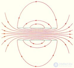
Fig. 6.24. The magnetic field of a coil of finite length
At the center of the solenoid the magnetic field is practically uniform and considerably exceeds in magnitude the field outside the coil
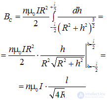
Solution. The magnetic field at the midpoint of the axis of a solenoid of finite length l is given by the same integral (6.19), but with different limits of integration
|
|
(6.21) |
If the length of the solenoid is much greater than its diameter (l >> 2R), we return to the formula for the field in an infinitely long solenoid (6.20). The relative difference between these two values equals
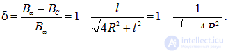
By condition this difference is small:  , that is, the ratio of the solenoid's diameter to its length is small: 2R/l << 1. Therefore we can use the formula for the expansion of the square root
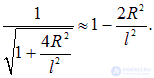
Hence

or

Substituting the numerical value of d, we find that the difference will be less than half a percent when the relation
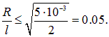
In other words, a solenoid can be regarded as infinitely long if its length exceeds its radius by a factor of twenty or more.
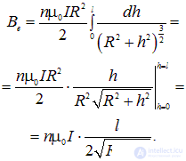
Example 2. Find the magnetic field Be at the extreme end point of the axis of a solenoid of finite length l. Compare with the result of the previous example.
Solution. The magnetic field at the end point of the axis of a solenoid of finite length l is given by the same integral (6.19), but now the limits of integration will look different
|
|
(6.22) |
The ratio of the fields at the middle and end points of the solenoid's axis equals
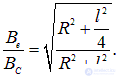
This ratio is always less than unity (that is, the field at the end is smaller than the field at the middle of the solenoid). At l >> R we have

This result is easy to understand. Let us imagine an infinite solenoid, which we mentally cut in half at the observation point. We can consider that the field at this point is created by two identical «semi-infinite» solenoids, located on opposite sides of it. It is clear that when one of them is removed, the observation point becomes the end of the remaining «semi-infinite» solenoid, and the magnetic induction at it decreases by exactly a factor of two.
This — is the so-called edge effect. This example demonstrates that it is not sufficient for the relation l >> R to hold in order to use the formulas for an infinitely long solenoid; it is also necessary that the observation point be far from its ends.
Fig. 6.25 shows an experiment studying the distribution of the magnetic field lines around a solenoid. The field of the solenoid, whose axis lies in the plane of the plate, is concentrated mainly inside the solenoid. Inside, the field lines look like straight lines parallel to the axis of the coil, while outside the field is practically absent.
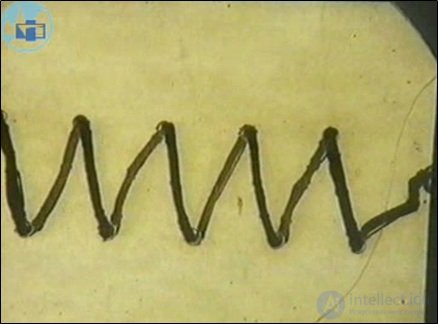
Fig. 6.25. Visualization of the magnetic field lines
Let us apply Ampère's law to calculate the force of interaction between two long straight conductors carrying currents I1 and I2, located at a distance d from each other (Fig. 6.26).
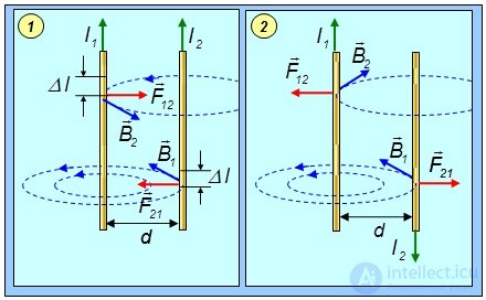
Fig. 6.26. Force interaction of straight currents:
1 — parallel currents; 2 — antiparallel currents
Video 6.2. Interaction of two parallel current-carrying conductors.
The conductor carrying current I1 creates a ring-shaped magnetic field, whose magnitude at the location of the second conductor equals
|
|
(6.23) |
This field is directed «away from us», orthogonal to the plane of the figure. The element of the second conductor  experiences the action of an Ampère force from this field
|
|
(6.24) |
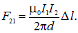
Substituting (6.23) into (6.24), we obtain
|
|
(6.25) |
For parallel currents, the force F21 is directed toward the first conductor (attraction); for antiparallel currents, in the opposite direction (repulsion).
Similarly, an element  of conductor 1 experiences the magnetic field created by the conductor carrying current I2 at the point in space containing the element , with a force F12. Reasoning in the same way, we find that F12 = –F21, that is, in this case Newton's third law holds.
Thus, the force of interaction between two straight, infinitely long, parallel conductors, calculated per unit length element of the conductor, is proportional to the product of the currents I1 and I2 flowing in these conductors, and inversely proportional to the distance between them. In electrostatics, two long charged filaments interact according to an analogous law.
Fig. 6.27 shows an experiment demonstrating the attraction of parallel currents and the repulsion of antiparallel ones. Two aluminum strips, suspended vertically next to each other in a loosely tensioned state, are used for this. When parallel direct currents of about 10 A are passed through them, the strips attract each other, while reversing the direction of one of the currents makes them repel.
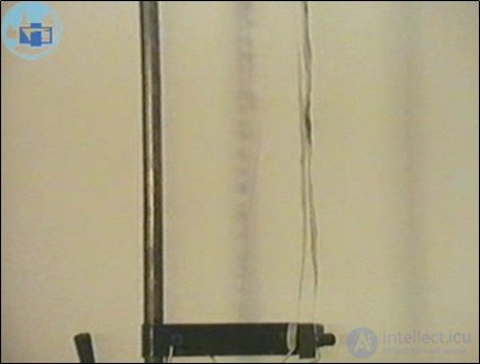
Fig. 6.27. Force interaction of long straight current-carrying conductors
On the basis of formula (6.25), the unit of current — the ampere, one of the base units in the SI — is established.
|
Ampere — the current of unchanging strength which, flowing through two long parallel conductors placed in vacuum 1 m apart, produces between them an interaction force of 2×10⁻⁷ N per meter of conductor length. |
Example. Two thin wires, bent into identical rings of radius R = 10 cm, carry identical currents I = 10 A each. The planes of the rings are parallel, and their centers lie on a straight line orthogonal to them. The distance between the centers is d = 1 mm. Find the interaction force between the rings.
Solution. One should not be confused by the fact that in this problem we know only the law of interaction of long straight conductors. Since the distance between the rings is much smaller than their radius, the interacting elements of the rings «do not notice» their curvature. Therefore the interaction force is given by expression (6.25), where instead of we must substitute the circumference of the rings  We then obtain

|
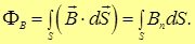
The flux of the magnetic flux density vector B (magnetic flux) through a small surface of area dS is the scalar physical quantity equal to
|
Here  ,
,  is the unit vector normal to the area of area dS, Bn is the projection of the vector B onto the normal direction,
  is the angle between the vectors B and n (Fig. 6.28).
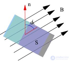
Fig. 6.28. Flux of the magnetic flux density vector through a surface element
The magnetic flux ΦB through an arbitrary closed surface S equals
|
|
(6.27) |
The absence of magnetic charges in nature means that the lines of the vector B have neither beginning nor end. Therefore the flux of the vector B through a closed surface must equal zero. Thus, for any magnetic field and any closed surface S, the condition holds
|
|
(6.28) |
Formula (6.28) expresses the Ostrogradsky — Gauss theorem for the vector  :
:
|
The flux of the magnetic flux density vector through any closed surface is identically equal to zero. |
Let us emphasize once again: this theorem is the mathematical expression of the fact that magnetic charges do not exist in nature, on which the lines of magnetic flux density could begin and end, as was the case for the electric field strength E of point charges.
This property fundamentally distinguishes the magnetic field from the electric field. Lines of magnetic flux density are closed, so the number of lines entering a certain volume of space equals the number of lines leaving that volume. If the incoming fluxes are taken with one sign and the outgoing ones with the other, then the total flux of the magnetic flux density vector through a closed surface will equal zero.
|
In the SI system, the unit of magnetic flux is the weber (Wb) (Fig. 6.29):
|
Fig. 6.29. W. Weber (1804–1891) — German physicist
The difference between the magnetic field and the electrostatic field also shows up in the value of the quantity we call the circulation — the integral of a vector field along a closed path. In electrostatics, the integral

taken along an arbitrary closed contour, equals zero. This is related to the potential nature of the electrostatic field, that is, to the fact that the work done in moving a charge in an electrostatic field does not depend on the path, but only on the position of the initial and final points.
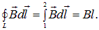
Let us see how matters stand with the analogous quantity for the magnetic field. Take a closed contour enclosing a straight current, and calculate for it the circulation of the vector B, that is

As was obtained above, the magnetic flux density created by a straight current-carrying conductor at a distance R from the conductor equals

Consider the case when the contour enclosing the straight current lies in a plane perpendicular to the current and represents a circle of radius R centered on the conductor. In this case the circulation of the vector B around this circle equals
|
|
(6.29) |
whence
|
|
(6.30) |
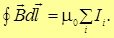
It can be shown that the result for the circulation of the magnetic flux density vector does not change under continuous deformation of the contour, provided the contour does not cross any current lines during this deformation. Then, by virtue of the superposition principle, the circulation of the magnetic flux density vector along a path enclosing several currents is proportional to their algebraic sum (Fig. 6.30)
|
|
(6.31) |
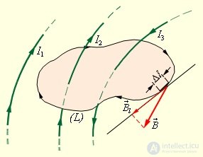
Fig. 6.30. A closed contour (L) with a given direction of traversal.
The currents I1, I2 and I3, creating the magnetic field, are shown.
Only the currents I2 and I3 contribute to the circulation of the magnetic field along the contour (L)
If the chosen contour does not enclose any currents, then the circulation  around it equals zero.
When calculating the algebraic sum of the currents, the sign of the current must be taken into account: a current will be considered positive if its direction is related to the direction of traversal around the contour by the right-hand screw rule. For example, the contribution of current I2 to the circulation is negative, while the contribution of current I3 is positive (Fig. 6.18). Using the relation

between the current I through any closed surface S and the current density  , for the circulation of the vector B we can write
|
|
(6.32) |
where S is any closed surface bounded by the given contour L.
Thus,
|
The circulation of the magnetic flux density is nonzero if the contour along which it is taken encloses a current. |
Such fields are called solenoidal. Therefore no potential can be introduced for the magnetic field, as was done for the electric field of point charges. The difference between a potential field and a solenoidal field can be seen most clearly from the pattern of field lines. The field lines of an electrostatic field resemble hedgehogs: they begin and end on charges (or go off to infinity). The field lines of a magnetic field never resemble «hedgehogs»: they are always closed and enclose the flowing currents.
To illustrate the application of the circulation theorem, let us find, by another method, the already known magnetic field of an infinite solenoid. Take a rectangular contour 1-2-3-4 (Fig. 6.31) and calculate the circulation of the vector B along this contour
|
|
(6.33) |
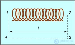
Fig. 6.31. Application of the circulation theorem for B to determining the magnetic field of a solenoid
The second and fourth integrals equal zero because of the perpendicularity of the vectors  and
and  . The third integral can be taken equal to zero, given the smallness of the magnetic field outside the solenoid. Therefore
|
|
(6.34) |
The contour considered encloses a total current nlI, where n is the number of solenoid turns per unit length, and I is the current strength in the solenoid. Consequently,

or
|
|
(6.35) |
We have reproduced result (6.20) without integrating the magnetic fields from individual turns.
The result obtained (6.35) can be used to find the magnetic field of a thin toroidal solenoid (Fig. 6.32).
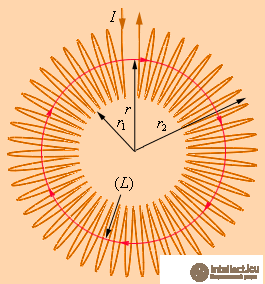
Fig. 6.32. Toroidal coil: the lines of magnetic flux density close up inside the coil and form concentric circles. They are directed so that, looking along them, we would see the current in the turns circulating clockwise. One of the flux density lines of a certain radius r1 ≤ r < r2 is shown in the figure
The connection between electricity and magnetism is not exhausted by the similarity of a number of relations. In essence, both of these fields are different manifestations of a single electromagnetic field. In the course on mechanics we spoke of the principle of relativity, that all laws of nature must be invariant under transition from one inertial reference frame to another. However, the electric and magnetic fields taken by themselves, separately, clearly do not satisfy this principle. Indeed, in an inertial reference frame K, take a charge q moving rectilinearly and uniformly with velocity v. It creates a Coulomb electric field and, in addition, a magnetic field whose flux density vector is given by expression (6.2). Let us attach to the charge a reference frame K ', which will also be inertial. In this reference frame the charge is at rest, and the field it creates will be purely electrostatic. It turns out that the electric and magnetic fields do not have an absolute character. Upon transition to another reference frame, they must transform into one another (Fig. 6.33).
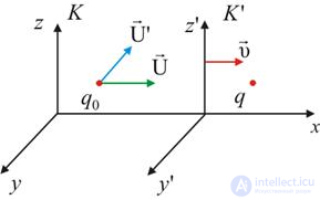
Fig. 6.33. A charge at rest in a moving reference frame
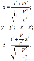
Let us recall the Lorentz transformations for spatial coordinates and time
|
|
(6.36) |
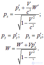
Let us not forget that similar transformations connect the momentum and energy of a particle in different reference frames
|
|
(6.37) |
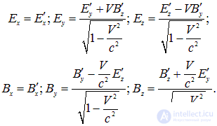
Shall we now be surprised that the electric and magnetic fields in different reference frames are also related by Lorentz transformations
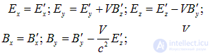
|
|
(6.38) |
Recall that primed quantities refer to the reference frame K ', which moves relative to the frame K along the x axis with velocity V.
From the Lorentz transformations it follows that the electric field of a moving charge is stretched in the direction perpendicular to the velocity (Fig. 6.34).
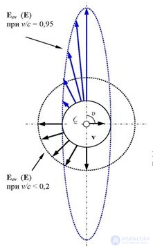
Fig. 6.34. Electric field of a moving charge
Note that the Lorentz transformation formulas for the electromagnetic field differ from the transformations for space-time or energy-momentum in that the field components along the line of motion of the reference frame K ' (that is, along the 0x axis) do not transform. To illustrate this, consider the laboratory reference frame K, in which there is an electric field E, but no magnetic field (B = 0). In what case will an observer in the moving reference frame K ' also observe only a purely electric field E ' with no admixture of a magnetic one (B ' = 0)? The answer follows from formulas (6.38) upon substituting zero values for B, B ': from the second equation it follows immediately that E 'y = E 'z = 0, and from the first — Ey = Ez = 0. In other words, this is possible when the electric field (not necessarily uniform) is directed along the motion of the reference frame K '.
The equations of electromagnetism were from the outset invariant with respect to these transformations, so that the theory of relativity fit quite painlessly together with electromagnetic theory, while classical mechanics underwent substantial revision. Instead of justifying the validity of transformations (6.38), which is beyond the scope of our course, let us get acquainted with one more of their consequences.
Since so far we are dealing mainly with nonrelativistic physics, let us simplify the Lorentz transformations for the case when the velocity of the reference frame K ' is much smaller than the speed of light: V << c. In this case, as already noted, the square roots

and transformations (6.38) take the form
|
|
(6.39) |
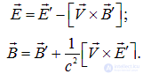
These equations can be written in vector form
|
|
(6.40) |
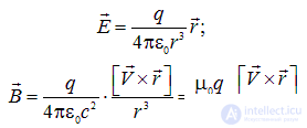
Let us return to our charged particle, at rest in the frame K '. In this frame there is no magnetic field (B ' = 0), and the electric field is given by Coulomb's law
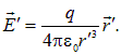
Since we assume V << c, we use the Galilean transformations for spatial coordinates and time intervals, so that the radius vector drawn from the particle to the observation point is the same in both reference frames: r = r '. Substituting the indicated expressions for B ', E ' into transformations (6.40), we obtain
|
|
(6.41) |
Here we used relation (6.3)

The first equation of (6.41) is the ordinary Coulomb field of charge q, the second is the magnetic field of a moving charge (6.2). Thus, even classical magnetism is a manifestation of relativistic effects. The electric and magnetic fields turn out to be inseparably linked with one another into a single electromagnetic field, whose specific manifestation depends on the reference frame.
Example. An airplane flies horizontally at a speed of 250 m/s in the Earth's magnetic field with a magnetic flux density of 50 μT, directed vertically downward. What electromagnetic field will the passengers of the airplane observe?
Solution. Let us direct the 0x axis of the laboratory reference frame K, attached to the Earth, along the airplane's route, so that its velocity is written as

Let us direct the 0z axis vertically upward, so that the magnetic flux density is described by the vector

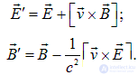
We need to find the electric and magnetic fields in the moving reference frame K ', attached to the airplane. Since the airplane's speed is much smaller than the speed of light, we can apply formulas (6.40). For convenience, however, we use the inverse formulas, obtained by replacing the primed quantities with unprimed ones and reversing the sign of the velocity: V = –v:
|
|
(6.42) |
Since in the laboratory frame there is no electric field (E = 0), it follows immediately from the second equation that B ' = B: the magnetic field for the airplane passengers will remain the same as for the relatives who saw them off on their flight. However, an electric field will also appear on the airplane. Its field strength, as follows from the first equation, equals
|
|
(6.43) |
Here we used the fact that the cross product of two unit vectors gives a third unit vector

Over a 60 m span, a potential difference  arises at its ends — a small quantity, but one accessible to measurement.



















Comments