
Lecture
Это продолжение увлекательной статьи про электрическое поле в вакууме.
...
first bump in early childhood, while Coulomb's law remains unknown to many of our fellow citizens even after finishing secondary school? The reason is that in the macroscopic world, as we have seen, the positive and negative electric charges in bodies are compensated, so that in ordinary life we deal with relatively small excess charges. At the same time, all gravitating masses have the same sign, so no compensation of masses occurs, and gravitational forces manifest themselves more strongly at the macroscopic scale.
An electric field can be specified by giving, for each point, the magnitude and direction of the electric field strength vector  . To visualize an electric field, field lines are used (or lines of the vector field ).
|
A line of electric field strength (field line) is a line whose tangent at each of its points coincides in direction with the electric field strength vector. |
Fig. 1.17 shows a field line of the electric field. The electric field strength vectors are directed along the tangent to the field line.
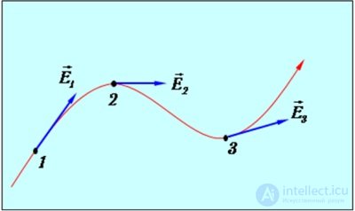
Fig. 1.17. Electric field strength vectors are directed along the tangent to the field lines
The number of lines passing through a unit-area patch perpendicular to them is proportional to the magnitude (modulus) of the electric field strength at that location. In other words, field lines are drawn more densely where the field strength modulus is larger. Thus, the configuration of field lines allows one to judge the change in direction and magnitude of the vector in space. The pattern of vector field lines (not necessarily electric or magnetic) is a very illustrative graphical way of displaying its basic properties.
Let us note some important properties of the field lines of an electrostatic field:
would be a multivalued function of the point's coordinates);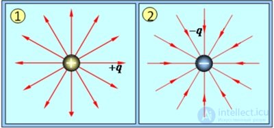
Fig. 1.18. Field lines of a point charge: 1 — q > 0; 2 — q < 0
In the first case, the field lines begin at the positive point charge and go off to infinity; in the second case, the field lines come from infinity and end at the negative point charge.
The field lines of the electric field created by two point charges of equal magnitude and like sign are shown in Fig. 1.19.
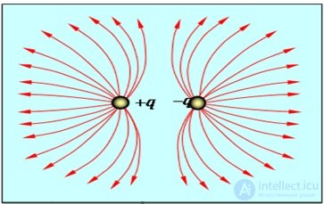
Fig. 1.19. Field lines of the electric field formed by two equal positive point charges
The pattern of field lines of the electric field created by two point charges of equal magnitude and opposite sign is shown in Fig. 1.20.
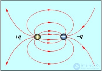
Fig. 1.20. Field lines of the electric field formed by two point charges of opposite sign and equal magnitude
Note that the system of two charges equal in magnitude and opposite in sign, shown (together with its field) in Fig. 1.20, is called an electric dipole.
Video 1.5. The pattern of field lines of a point charge, of two identical point charges, and of a dipole — two point charges of opposite sign and equal magnitude (paper «tassels»).
Video 1.6. The pattern of field lines of a point charge, a dipole, and a cylindrical capacitor (semolina grains in castor oil).
|
An electric field whose strength is the same in magnitude and direction at all points in space is called a uniform electric field. |
The density and direction of the field lines remain unchanged throughout the entire volume of a uniform electric field. Such a field is graphically represented by parallel straight lines equally spaced from one another.
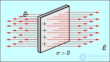
It will be shown later that an infinite uniformly charged plane creates a uniform electric field around itself. The field strength lines are directed perpendicular to the charged plane and point away from it if the plane is positively charged, and toward it if the plane is negatively charged (see Fig. 1.21).
|
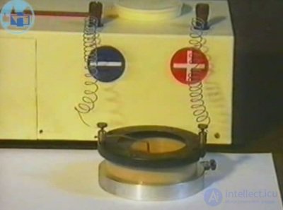
Fig. 1.21. Electric field of a uniformly positively charged plane The field lines of an electric field can be studied experimentally using the setup shown in Fig. 1.22. Electrodes connected to a high-voltage source are immersed in castor oil containing a suspension of small dielectric particles. When voltage is applied to the electrodes, the particles line up in chains along the field lines and show the distribution of the field in the space between the electrodes. By using electrodes of various shapes, one can study the field of point charges of the same and of different signs, the field of a parallel-plate and of a cylindrical capacitor, and so on.
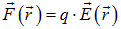
Fig. 1.22. Experimental study of the field lines of an electrostatic field The behavior of a charge in a given electric field is described by Newton's second law
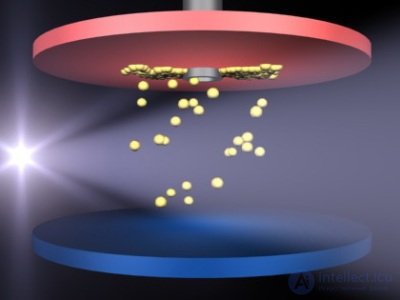
(Here it is assumed that no other forces act on the charge; otherwise, the corresponding terms would need to be added to the right-hand side). One of the methods for determining the charge of the electron (Millikan's method) is based on observing the motion of oil droplets in the vertical electrostatic field of a parallel-plate capacitor (Fig. 1.23). An electric field was created in the space between the two plates of the capacitor. Oil droplets were sprayed into this space. Under the action of light, the air between the plates was ionized, and the free electrons thereby produced were captured by the droplets, charging them.
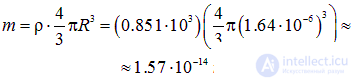
Fig. 1.23. Diagram of Millikan's experiment The motion of a droplet of radius 1.64 μm and density 0.851 g/cm3 was observed. It was noted that the droplet stopped falling when the electric field strength was 1.95·105 V/m. This meant that the electrostatic force qE balanced the force of gravity mg. The mass of the droplet is
|
From this we find the charge of the droplet
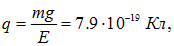
that is, the droplet carried five electron charges. It was precisely in such experiments that the quantization of electric charge was discovered and its minimal value e was determined.
The motion of charged particles can be controlled with the help of an electric field of the required magnitude and direction. This is what happens, for example, in the cathode-ray tube of an oscilloscope.
Fig. 1.24 shows the motion of an electron beam drawing a sine wave on the screen of a cathode-ray tube with electric deflection. In an oscilloscope, the amplified signal under study is applied to the vertical deflection plates, while a sawtooth sweep voltage is applied to the horizontal plates. As a result, the electron beam «draws» the dependence of the signal under study on time on the oscilloscope screen.
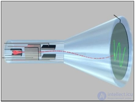
Fig. 1.24. Operating principle of a cathode-ray tube
The definition of the field strength is very often used in the form
|
|
(1.10) |
By virtue of the definition (or, equivalently, it is the same thing), the electric field strength is called its force characteristic — it determines the force acting on a charge placed in the field.
Example 5. A particle moving parallel to the plates along the axis of a parallel-plate capacitor flies into the space between the plates (Fig. 1.25). The particle acquired its initial kinetic energy by passing through an accelerating potential difference  Under the action of the capacitor's field, the particle is deflected toward one of the plates (depending on the sign of its charge) and eventually strikes it. This distance
  can be measured. Also known are the distance
  between the plates and the voltage
  across the capacitor. Can these data be used to determine the type of particle (by finding its specific charge, i.e., the ratio of the charge
  to the mass
  )?
)?
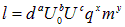
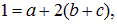
Solution. Let us first solve the problem by the method of dimensional analysis. The distance traveled must be a function of the parameters of the problem:
|
|
Recalling that the product of the potential and the charge gives energy, whose dimension is 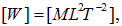 we obtain
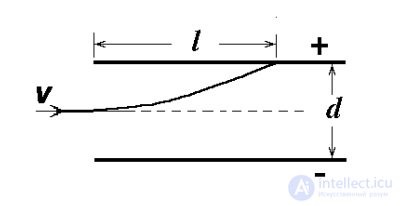
Fig. 1.25. Motion of a charged particle between the plates of a parallel-plate capacitor
Substituting this dimension, we obtain the equation:
|
|
Comparing the dimensions on both sides of the equality, we arrive at the equations:
|
|
|
The last equation, following from the absence in the left-hand part of a quantity with the dimension of time, immediately gives us  or
or  After that we immediately find:
  Substituting the values found, we obtain:
|
|
|
The arbitrary power (the exponent b could not be determined) means that the result depends on an arbitrary function of the dimensionless ratio 
|
|
|
We do not yet know the form of this function: if the problem involves quantities of the same dimension, then, naturally, the function of their ratio cannot be found by dimensional analysis. But we can already answer the question of the problem: the parameters characterizing the particle — neither its mass nor its charge — entered into the answer. All particles under the given conditions will be deflected equally, and such a device cannot be used to identify them.
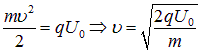
Let us now give the exact solution of the problem. We find the initial velocity of the particle from the relation
|
|
|
In the capacitor, the particle is under the action of the electric field  and acquires a transverse acceleration
 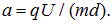 It will cover the distance
  before striking the plate in a time t:
|
|
|
from which we find the flight time:
|
|
|
In the longitudinal direction, during this time the particle will travel a distance
|
|
|
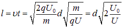
We arrive at the same conclusion about the independence of  from the characteristics of the particle. Moreover, we have now found the function
  which was left undetermined in our preliminary result.
In Chapter 4 of the section «Mechanics» it was shown that a conservative force  is related to the potential energy
  by the relation
|
|
(1.11) |
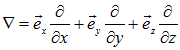
Here the symbol  — is the generally accepted notation for the vector operator «nabla», whose action on a scalar function of coordinates yields the gradient of that function. The explicit form of the nabla operator in Cartesian coordinates is as follows:
|
|
(1.12) |
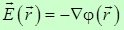
Substituting into  and dividing by
  , we obtain
|
|
(1.13) |
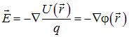
The scalar function  is called the electric field potential.
|
The function
is called the electrostatic field potential. |
As can be seen from (1.13), the potential energy of a point charge  in a field with potential
  is equal to
|
|
(1.14) |
and the force acting on it 
|
|
(1.15) |
In Supplement 3, an example of the use of these relations is worked out.
|
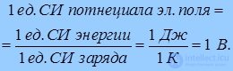
In SI, the unit of measurement of electric field potential is the volt (V):
|
The field strength determines the force acting on a point charge in the field, while the potential determines its potential energy in that field. Therefore, following the meaning of these relations, the electric field strength  is called the force characteristic of the field, and the potential
  — its energy characteristic.
Like the potential energy, the field potential is always defined up to an additive constant. This is evident from the fact that, since nabla is a differential operator, the potentials  and
and 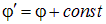 are physically identical, since they correspond to a field of the same strength
 .
.
This allows one to normalize the potential by arbitrarily choosing some point  and setting the potential at that point equal to zero
|
|
(1.16) |
Given that both the field strength and the field potential decrease as the distance  to the system of charges creating the field increases, in all those cases where a finite
  charge is distributed over a finite region of space, it is natural and convenient to normalize the potential to «zero at infinity», that is, to set it equal to zero at an infinite distance from the system of charges
|
|
(1.17) |
Those idealized cases in which normalization to zero at infinity is, precisely because of the idealization of the problem, meaningless, will be discussed later.
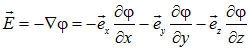
Relation (1.13) makes it possible to compute the field strength from a known potential;
|
|
(1.18) |
Let us obtain the «inverse» relationship: let us express the field potential in terms of its strength. To do this, let us compare three expressions: the expression for  from (1.18), the expression for the vector of an infinitesimal displacement
  , and the expression for the total differential
  of the function
  :
:
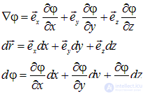
It is easy to see that the scalar product of the first two vectors is equal to the total differential  of the potential
|
|
(1.19) |
or, taking into account
|
|
(1.20) |
In fact, this relation is not new. If we multiply (1.20) by the charge  and take into account relations (1.14) and (1.15), we obtain the relation, familiar from Chapter 4 of the section «Mechanics», connecting the work of a conservative force and the decrease in potential energy
 .
.
Also in the section «Mechanics» it was shown that a stationary potential field is conservative. From relation (1.18) it follows that the electrostatic field is conservative in all those cases where the field potential does not depend on time.
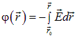
Integrating relation (1.20) from the point  , at which the potential is taken to be zero, to some point
  , at which we are interested in the potential, along an arbitrary curve convenient for the calculation (the field is conservative and the result does not depend on the shape of the curve), we obtain
|
|
(1.21) |
Let us use (1.21) to compute the field potential of a point charge  located at the origin of coordinates, normalizing it to zero at an infinite distance from this charge. For this we shall use Coulomb's law in the form (1.9):
|
|
(1.22) |
In this calculation, the identity  was used, valid for any vector
  :
:  and being the result of simple differentiation of the definition of the modulus of any vector:
  .
.
Thus, the potential of the field of a point charge located at the origin of coordinates has the form
|
|
(1.23) |
and this field, as already noted earlier, is central: in fact the field potential depends only on  .
.
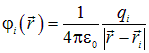
Given that the modulus of the radius vector  standing in the denominator is nothing other than the distance from the charge creating the field to the field observation point, the formula is easily generalized to the case where the charge
  is located not at the origin of coordinates, but at a point with radius vector
  . In this case, the distance from the charge to the field observation point is equal to
  and the field potential at the point
  (with the same normalization to zero at infinity) is equal to
|
|
(1.24) |
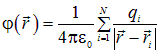
The relationship between the field strength and its potential  is linear, so the superposition principle for the field strength is also valid for the field potential. In other words: the potential of the field of a system of charges is equal to the algebraic sum of the potentials of the field from each of the charges of the system. Using the superposition principle, the potential of the field of a system of charges can be written down at once
  :
:
|
|
(1.25) |
Here  — is the total number of charges in the system.
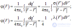
In the case of a continuous distribution of charge over some volume  , we obtain
|
|
(1.26) |
For a continuous distribution of charge over some surface  or curve
  , we obtain respectively
|
|
(1.27) |
where  and
and  — are the corresponding surface and linear densities.
In Supplement 4, an example of the use of the relations just obtained is worked out.
We shall not consider separately here the question of the work of electrostatic forces when point charges and charged bodies are moved in an electrostatic field. The electrostatic field is conservative (Fig. 1.26), the potential energy of a charge in the field is equal to 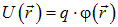 , so the work of electrostatic forces can always be computed with the help of relations of the form

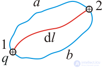
Fig. 1.26. The work of electrostatic forces depends only on the positions of the initial and final points
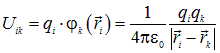
Let us compute the interaction energy of the charges making up some system.
To number these charges it is convenient to use two indices, for example,  and
and  . The same charges of the system, once denoted this way, this is
 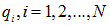 , another time this is
 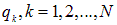 . Let us emphasize that the charge
  and the charge
  are one and the same 5th charge of the system. Such «complications» are necessary for a compact notation of the expression for their interaction energy, and here is why. Charges interact pairwise, and the interaction energy of the
  and
and  charges is equal to
|
|
(1.28) |
Here  — is the potential of the
  charge at the point where the
  charge is located.
In  — we do not consider the interaction of a charge with itself, or its potential energy in its own field.
Therefore, when summing the energies of the pairwise interactions of charges, we must necessarily take into account that  , firstly, and, secondly, that each pair of charges must appear in the sum only once. This can be done in two ways. The first consists in explicitly stipulating, when writing the double sum, for example, that
  :
:
|
|
(1.29) |
In the second method, while maintaining the inequality  , summation is carried out over all possible values of
  and
and  , respectively, and the term corresponding to the interaction of one and the same pair of charges appears in the sum twice, so the sum must be divided by 2. We obtain:
|
|
(1.30) |
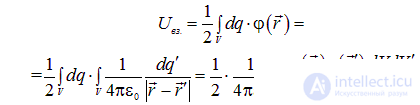
In the case of a continuous distribution of charge over some volume  with density
  , the relation, for example, takes the form:
|
|
(1.31) |
In the first of the formulas in (1.31),  — is the potential of all charges except
  at the point
  where
where  is located; in the second relation this potential is written out explicitly; in the third, the following operation has been performed: two integrals have been combined into one for brevity, and the charges and
  have been expressed in terms of the charge density
  .
.
We shall not write out here the formulas for the cases of a charge distributed over a surface or along some curve; they only require replacing  with
with  and
and  .
.
For a visual representation of the distribution of potential in space, equipotential surfaces are used.
|
An equipotential surface (surface of equal potential) — is the set of points having equal potential. |
Let us consider the pattern of equipotential surfaces of some fields.
Recall that both from physical considerations and directly from the relation  follows the mutual orthogonality of field lines and equipotential surfaces. Indeed, by definition, the equation of an equipotential surface has the form
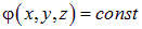
Differentiating this relation, we obtain

for all displacements  , tangent to the equipotential surface. This means the vector
  is perpendicular to the equipotential surface. It remains to recall that the vector
  is directed along the tangent to the field line by definition. The statement about the orthogonality of field lines and equipotential surfaces is proved.
The equipotential surfaces of the field of a point charge are concentric spheres centered at the point where the charge is located (see Fig. 1.27). The equipotential surfaces are marked with solid blue lines, and the field lines — with red dashed lines.
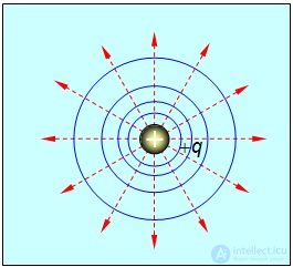
Fig. 1.27. Equipotential surfaces (spheres) (solid blue lines) and field lines (dashed red lines) of the field of a point charge
The equipotential surfaces of a uniform electric field are planes perpendicular to the field lines and located at equal distances from one another (see Fig. 1.28).
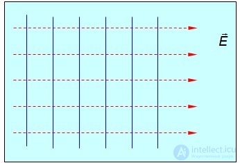
Fig. 1.28. Equipotential surfaces of a uniform electric field
The equipotential surfaces of the field of two identical like point charges are shown in Fig. 1.29.
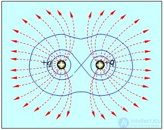
Fig. 1.29. Equipotential surfaces of two identical like point charges
The equipotential surfaces of the field of two point charges of opposite sign and equal magnitude are shown in Fig. 1.30.
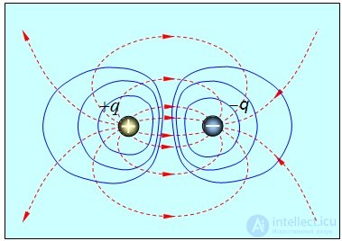
Fig. 1.30. Equipotential surfaces of two point charges of opposite sign and equal magnitude
A graphical view of the two-dimensional (in the plane z = 0) electric field potential created by a point charge located at the origin of coordinates is shown in Fig. 1.31.
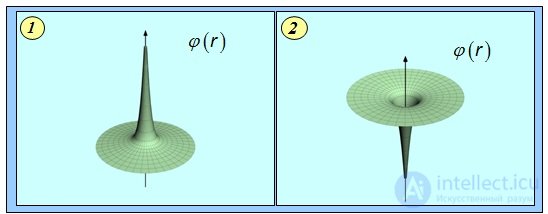
Fig. 1.31. View of the two-dimensional (in the plane z = 0) Coulomb potential 1/r near a positive (1) and a negative (2) point charge. In case (1), a positive test charge runs into an infinitely high potential barrier preventing penetration to the center. In case (2), an attractive force acts on the test charge, and it tends to roll down into the resulting potential well
An experimental study of the field potential around a charged metal sphere using a «flame» probe is shown in Fig. 1.32. The probe used is connected to an electrometer. To equalize the probe's potential with the potential of the point where it is located, the measuring probe is placed in the flame of a small gas burner, which ionizes the air and allows charge to flow onto and off the probe. This demonstrates the decrease in potential as the probe is moved radially from the center of the sphere, and the constancy of potential as the probe is moved along a circle around the center of the charged sphere.
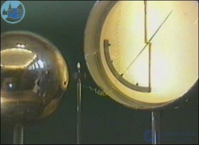
Fig. 1.32. Experimental study of the field potential around a charged metal sphere using a «flame» probe
In Supplement 7, a useful relation is derived for the gradient of a scalar function depending only on the modulus of the radius vector.
The theorem was established by M.V. Ostrogradsky (Fig. 1.33) in the form of a general mathematical theorem for any vector field, and by K. Gauss — as applied to the electrostatic field.
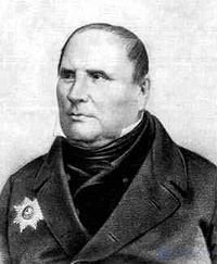
Fig. 1.33. M. Ostrogradsky (1801–1861) — Russian mathematician and mechanician
Coulomb's law and the superposition principle make it possible to compute the field potential of any charge distribution
 .
.
Using the relation 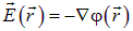 or directly with the help of Coulomb's law and the superposition principle, one can also compute the field strength

However, the practical computation of the sums and integrals written above is far from always as simple as the sums and integrals themselves appear. They are computed quite easily when there are two, three, perhaps a dozen charges. But if we are dealing with macroscopic charged bodies, when the number of point charges (protons, electrons, etc.) is macroscopically large, the direct computation of such expressions becomes a very difficult task. This applies primarily to the sums written above, and not to the integrals.
We wish to emphasize that when solving macroscopic problems, in the overwhelming majority of cases, the charge can be considered to be distributed continuously, and accordingly, one must compute not sums but integrals. Therefore the task arises: on the basis of Coulomb's law and the superposition principle, to write integral and/or differential equations satisfied by the field strength of an arbitrary distribution of charges. This task is, in a number of cases, successfully solved by Gauss's theorem for the vector  , discussed in this section.
Let us consider some surface  and, on it, an infinitesimal patch (an infinitesimally small area element) of area
  (Fig. 1.34).
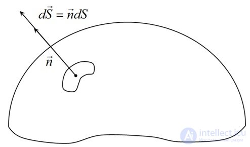
Fig. 1.34. An infinitesimal element of a surface
Shown in the figure, the «area vector»  has the following meaning: 1) it is directed along the normal
  to the surface
  at that point of it near which the area element is located; 2) its modulus is equal to the area of the element
  . The vector
  , and along with it the vector
  are always directed along the perpendicular to the surface at that location, but in which direction: to the upper left, as in the figure above, or in the opposite direction (to the lower right, «under» the surface) — in the general case this is a matter of arbitrary choice. However, in a number of cases, by default, certain rules apply. For example, if the surface is closed, that is, it represents a certain closed «shell», then by default the «outer» normal, directed outward, is taken. The choice of the «inner» normal contradicts nothing, but must be specifically stipulated. If the surface is not closed and rests on some contour, and, moreover, a direction of traversal of this contour is given, then the direction of the normal is generally accepted to be related to the direction of traversal by the right-hand screw rule. With the same reservation as above: the direction of traversal of the contour and the direction of the normal to the surface resting on it can be related using a left-hand rather than a right-hand screw; such a choice contradicts nothing, but must be specifically stipulated. Here and below, unless otherwise specifically stated, the above generally accepted rules will be used: the outer normal and the right-hand screw.
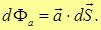
Let us introduce the flux  of an arbitrary vector
  through the chosen area element. By definition:
|
The flux
|
Formally, an infinitesimally small area element is considered; in practice (for example, in numerical summation) it must be small enough that the vector  can be regarded as constant (uniform) within its bounds, and the area element itself as flat, so that no ambiguity arises as to at which point within the element the normal should be drawn.
For generality of the definition (in physics, fluxes of other vectors are also considered), an arbitrary vector was considered above; as applied to the electric field strength vector  , taking into account the remark about the size of the area element, the definition of flux is illustrated in Fig. 1.35.
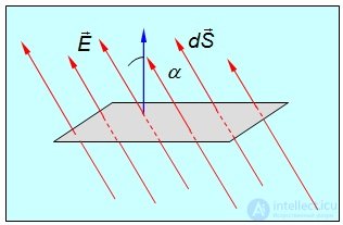
Fig. 1.35. Flux of the electric field strength vector through an infinitesimally small area element
According to the definition, the flux of the field strength vector through the area element equals (here and below, for brevity, when convenient, we will write «area element» and specify the vector of that element, which fully determines both its area and its orientation):
|
|
(1.43) |
where α — is the angle between the vectors  and
and  ,
,  — is the component of vector normal to the surface. Note that reversing the direction of the normal , just as reversing the direction of the field strength vector, changes the sign of the flux to the opposite one; thus, the flux of a vector is an algebraic quantity.
The flux of vector through an arbitrary surface S equals the sum of the fluxes through all the area elements into which the
продолжение следует...
Часть 1 1. The electric field in vacuum
Часть 2 1.4. Flux of a vector. The Ostrogradsky–Gauss theorem for a
Часть 3 1.5. Application of Gauss's theorem for calculating the electric field
Часть 4 Appendices - 1. The electric field in vacuum
Часть 5 - 1. The electric field in vacuum







 , related to the electrostatic field strength by the relation
 ,
,










 of the vector
  through an infinitesimal area element
  is the scalar product of the vector
  :
:


Comments