
Lecture
Now that we have such a powerful weapon as the Schrödinger equation in our hands, it is natural to return to the atom, starting with the simplest one — the hydrogen atom. After all, we need to make sure that quantum mechanics leads to the same results as the semiclassical Bohr theory of the atom. Moreover, there is hope that the new theory will present us with unexpected discoveries. It is only a pity that the study of methods for solving the Schrödinger equation lies outside the scope of this course. But that is not a problem: we will try to manage without excessive mathematics, guessing the properties of solutions on the basis of intuition developed while studying classical physics. At the same time, of course, no one intends to deceive the reader: everything «guessed» can be obtained from the Schrödinger equation by exact mathematical calculations.
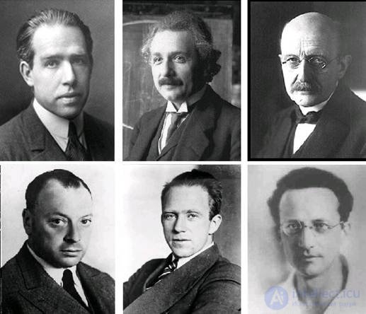
Fig. 5.1. Physicists who made a major contribution to the development of quantum mechanics at its early stage: (left to right) Niels Bohr, Albert Einstein, Max Planck, Wolfgang Pauli, Werner Heisenberg, Erwin Schrödinger
In the previous chapter we established that classical dynamical variables are replaced in quantum mechanics by operators acting on the wave function. The results of measuring some quantity A will always be the eigenvalues  of the corresponding operator

If the system is in some eigenstate  of the operator
  , then the measurement is certain to give the eigenvalue
  . If, however, the system is in some other state, then measuring the quantity A gives one of the eigenvalues with a certain probability, and this probability depends on the wave function of the state and, of course, on the quantity A.
Suppose the system is in a state with a definite value of the quantity A. This means that its wave function is an eigenfunction of the operator  . Can another quantity B also have a definite value? In other words, can the state be an eigenstate simultaneously for the operator
  , and for
  ?
?
Rule 3
|
Two operators
|
In other words: if the result of the sequential action of two operators does not depend on the order in which they are applied, then the corresponding quantities can simultaneously have definite values.
Let us consider an example
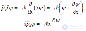
that is, for any function 

or simply

|
Since the operators |
This conclusion is precisely the true source of Heisenberg's uncertainty relations, whose physical meaning was discussed above.
The property of operators commuting with the Hamiltonian, that is, with the operator of the total energy  , is of special significance. If some operator
  commutes with , then there exists a common eigenstate, which is stationary by definition. In a stationary state the system remains for an unlimited time. This simultaneously means that the quantity A is conserved. Thus, the statement that some quantity is conserved is equivalent to saying that it can have a definite value together with the energy, that is, that its corresponding operator commutes with the Hamiltonian.
In classical mechanics, the angular momentum of a particle (also called the moment of momentum) is expressed as the vector product of the radius vector and the particle's momentum:

The same relation holds for operators in quantum mechanics:
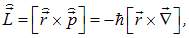
or in components
|
|
|
(5.1) |
and similarly for the other components
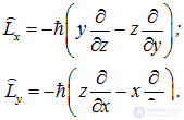
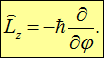
It was discussed earlier why the operator for the projection of angular momentum onto some axis is related to the derivative with respect to the angle of rotation about that axis (see equation (4.16)). In spherical coordinates, a rotation about the z axis is equivalent to a shift in the azimuthal angle  , and so the operator (4.1) has a particularly simple form
|
|
|
(5.2) |
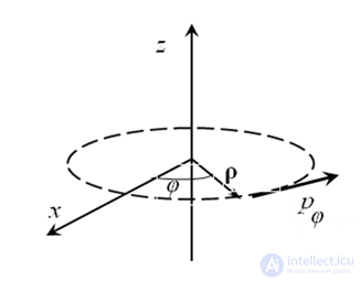
Fig. 5.2. The projection of angular momentum  is determined by the azimuthal component of momentum
The expressions for the other components  and
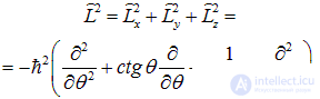
and  in spherical coordinates are quite complex, and here we will write out only the operator of the squared angular momentum
|
|
|
(5.3) |
Expression (5.3) is also fairly complex, and we will practically never use it. But even just by looking at it, we can already draw important conclusions
|
Instead of a formal mathematical proof of this last statement, let us point out the source of this property. Recall that  ,
,  and
and  are the operators of rotation of the system about the x, y, z axes, respectively. But the result of two such rotations depends on their sequence (Fig. 5.3), which is why the operators do not commute with one another.
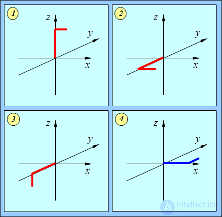
Fig. 5.3. Illustration of the non-commutation of the operators  ,
,  ,
,  ;
;
An L-shaped figure (1) is first rotated by 90° about the x axis (2), then — about the y axis (3).
With the reverse sequence of the same rotations the final result comes out different (4)
From what has been said an important consequence follows: only the square of the angular momentum and one of its projections can be measured simultaneously (usually chosen to be  ). This means that the vector L in quantum mechanics does not have a definite direction and cannot be regarded as a classical vector with three definite components. Thus, the «quantum angular momentum» can be conventionally pictured as a vector of fixed length (a definite value of the squared angular momentum), directed at a fixed angle to the z axis (a definite value of the projection), but precessing about this axis (the other components being undefined). This is nothing more than a mechanical analogy (the so-called vector model), but it correctly reflects the essential properties of angular momentum in quantum mechanics.
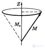
Fig. 5.4. Model of a precessing quantum angular momentum
Let us now find the eigenfunctions and eigenvalues of the operator  . We have the equation
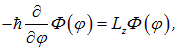
whence
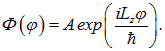
Note that here  (without the hat) is a number, not an operator.
Upon rotation through an angle  the system returns to its original state. For the wave function
  to remain unchanged, the following condition must hold

where m — is an integer (not necessarily positive). The constant A is determined by the normalization condition: the integral of the function
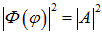
with respect to the angle  , ranging from 0 to
  , must equal unity
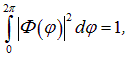
from which it follows that

Thus we arrive at the quantization condition for the projection of angular momentum:
|
The projection of angular momentum
|
The number m is called the magnetic quantum number. The eigenfunction of the operator  , corresponding to a given value m, has the form
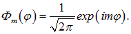
Essentially, the wave function  describes a plane wave running around a circle. The role of the coordinate is played by the angle
  , and the role of the wave vector — by the magnetic quantum number m. But the values of the variable are limited to the range between 0 and
  . Our «circular» wave is, as it were, confined in a potential well and undergoes finite motion. Hence — the quantization of the projection of angular momentum, in accordance with the laws of quantum mechanics established above.
Let us now find the quantization rules for the square of the angular momentum. Solving the corresponding equation for the eigenfunctions of the operator  is quite complex, and we will replace it with less rigorous but simpler considerations. Suppose that in some system the maximum value of the magnetic quantum number m equals a non-negative integer l. Then the minimum value n, obviously, equals –l, so that m runs through 2l + 1 possible values:

In the classical case, the maximum possible projection of angular momentum coincides with the magnitude of the vector  . But one should not expect the operator
  to have eigenvalues
  . We already know that even at the maximum value of the projection, the angular momentum is not parallel to the z axis (otherwise all three components of the momentum would be known). Consequently, the eigenvalues of the operator must be greater than
  . What, then, are they equal to?
If there is no distinguished direction in space, then any value of n is equally probable, and the mean value of the squared projection of the momentum onto the z axis equals
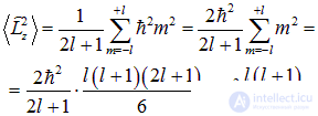
In deriving this, the well-known formula for the sum of squares of integers was used.
Note that all three coordinate axes are equivalent, so the same result holds for the mean values of the squares of the other projection operators of angular momentum:
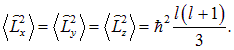
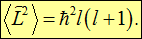
But their sum gives the squared angular momentum operator, whose mean value is thus equal to
|
|
|
(5.5) |
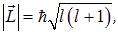
It is precisely this formula that describes the eigenvalues of the squared angular momentum operator, so that one can conventionally regard the length of the vector  in quantum mechanics as equal to

The non-negative integer quantum number l is called the azimuthal quantum number.
For comparison, let us obtain the classical answer in the same way. If l — is the maximum value of  for the classical vector, then
  runs through a continuous range of values from –l to l with equal probability dm/2l. The difference is that, because of continuity, the sum is replaced by an integral, and we obtain

and similar expressions for the two other means. Adding them, we arrive at the usual result of classical physics

For large values of l both results coincide (once again — the Bohr correspondence principle).
The main result of this section — is our acquaintance with the quantization rules for angular momentum: the eigenvalue of the squared angular momentum is determined by the value of the azimuthal quantum number l, while the projection of angular momentum — by the value of the magnetic quantum number m, which can take any of the values

If one nevertheless tries to picture the «quantum vector» of angular momentum as an ordinary vector, one can say that, for a given length of this vector, it makes only strictly defined angles with the distinguished axis (Fig. 5.5).
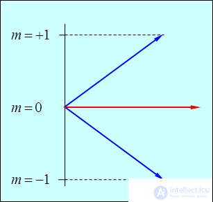
Fig. 5.5. Possible orientations of the angular momentum vector for l = 1:
the length of the vector is 1.41, and its projection onto the selected axis can take only the values 0 and +1 (in units of  )
)
Let us emphasize once again that this picture — is nothing more than an attempt to depict quantum properties in classical terms.
Example. Let us show that, according to quantum mechanics, the direction of the angular momentum  cannot coincide with a distinguished direction in space, and that in the limit of large azimuthal numbers
  the classical properties are restored.
Since the magnitude of the angular momentum vector takes the values
and its projection onto the distinguished direction equals

we can introduce the angle  between the direction of the angular momentum and the distinguished axis, so that
  will take only definite values
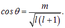
It follows that the minimum value of the angle  is determined by the maximum value of its cosine, attained at m = l:
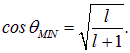
It is clear that for any finite value of l the angle is nonzero. For example, for states with l = 1 we obtain
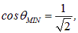
that is  , while for states with l = 3 we have
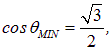
and  . It is clear that as l increases, the minimum angle between the angular momentum and the axis decreases, and in the limit

we obtain  . This is precisely the classical property of angular momentum: the ability to be exactly parallel to any distinguished direction.
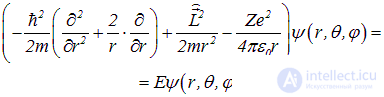
The stationary Schrödinger equation for a hydrogen-like atom (one electron near a nucleus of charge Ze) has the form

It is convenient to write this equation in spherical coordinates:
|
|
|
(5.6) |
Of course, we will not solve this equation, but simply take a careful look at it.
Note that the part of equation (5.6) that depends on the angles enters only through the operator of the squared angular momentum (5.3). The physical meaning of this term is fairly clear. Imagine that, in a central-force field, along an orbit of radius r there moves a classical particle with momentum  . Its angular momentum equals
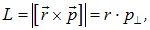
where  — is the projection of the momentum onto the direction orthogonal to the radius vector
  . Let us denote

the kinetic energy of the «orthogonal» motion. It can be expressed in terms of the squared angular momentum:

This term is added to the potential energy of Coulomb attraction to the nucleus, and it can be interpreted as the potential energy in a field of centrifugal forces. Indeed, if  — is the potential energy, then its derivative with respect to r should give the corresponding forces:

In the resulting expression one can easily recognize the formula for the centrifugal force known from classical mechanics. Quantum mechanics, as it should, reproduces at a new level the results of classical mechanics: now the angular momentum has become an operator, but it enters, on the same footing as before, into the expression for the operator of the total energy (the Hamiltonian).
Any operator commutes with itself, and since the operator of the squared momentum (5.3) does not depend at all on the radial variable r, then

commutes with the Hamiltonian (5.6). In addition, the operator for the projection of angular momentum

commutes with

and hence with the Hamiltonian. Consequently, the classical conservation laws for the square and one projection of the angular momentum hold. These conservation laws are valid for any centrally symmetric field: the specific nature of the Coulomb interaction has not yet been used. Therefore the projection and the square of the momentum can be determined simultaneously with the energy, and the wave function of the stationary state will depend on the quantum numbers l and m. However, in the Schrödinger equation (5.6) the Hamiltonian does not depend at all on the operator for the projection of angular momentum. This means that the energy of the state will not depend on the magnetic quantum number m. In other words, in any centrally symmetric field there is a degeneracy with respect to n, whose multiplicity equals 2l + 1. We already know that the source of degeneracy must be some symmetry or other. In classical physics, the motion of a particle in a centrally symmetric field always takes place along an orbit lying in a single plane. But this plane itself can be arbitrary, depending on the initial position and velocity of the particle. It is clear that the value of the particle's total energy does not depend on the orientation of the orbital plane in space. This is precisely the symmetry we are looking for, which leads to the degeneracy with respect to the magnetic quantum number.
In the Coulomb field (as well as in the gravitational field) there is one more specific degeneracy, which leads to the energy of the system not depending on the quantum number l either.
Let us again recall classical physics. In the Coulomb field, finite motion of a particle takes place only along an ellipse. Let us take an artificial satellite as an analogy. Let us place it at some distance from the Earth (that is, let us fix the potential energy) and give it some speed (let us fix the kinetic energy). We have thus fixed the total energy of the satellite. But is its orbit determined? Of course not! At the same total energy, the direction of the velocity affects the shape of the orbit — from a straight line (vertical fall) at zero angular momentum, to a circle of the maximum possible radius at a given total energy. Zero angular momentum corresponds to purely radial oscillations through the center of attraction, when there is no circular motion at all, and the ellipse degenerates into a straight line (for a satellite such an oscillation is impossible, but for microparticles — it is a different matter). The maximum possible angular momentum is attained in the opposite case of a purely circular orbit, when there is no radial motion at all. It is important that its (the maximum angular momentum's) magnitude depends on the total energy of the satellite.
Let us emphasize that the upper bound on the possible value of the angular momentum  — for a given total mechanical energy
  — has a purely classical origin. This can be verified as follows. Let us write the classical (non-quantum) expression for in the form
 .
.
Here  — is the kinetic energy of the radial motion:
  – is the radial component of the velocity,
 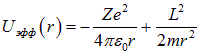 — is the effective potential energy, which includes the potential energy in the field of centrifugal forces. It is clear that
  . Taking into account that the energy of bound states is less than zero, let us rewrite this inequality in the form
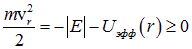
or
 .
.
The effective potential energy, for a nonzero angular momentum L, has a minimum at the point 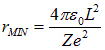 , and its minimum value equals
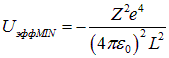 .
.
Since the inequality  must also hold at the minimum point, we obtain
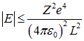 or
or 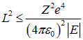 .
.
If we substitute into this last inequality the Bohr expression (3.3) for the energy of a hydrogen-like ion and the expression (5.5) for the squared angular momentum, we obtain the inequality
 ,
,
which has the solution
 .
.
Here n — is the Bohr number of the stationary orbit, or the principal quantum number (see below). The rigorous quantum theory, based on solving the Schrödinger equation (5.6), gives the same result.
Thus, classical physics suggests to us the following properties of the solutions of the Schrödinger equation:
|
Armed with knowledge of classical mechanics, we can now confidently proceed to the study of quantum mechanics. The properties of the solutions of the Schrödinger equation for the hydrogen atom will now become clear. Its solutions are wave functions labeled by three quantum numbers:  . Much has already been said about l and n , and n — is the principal quantum number familiar to us from the Bohr atom, taking positive integer values. Different sets of numbers correspond to different wave functions, whose general form — for any possible sets of numbers – is not important for us right now.
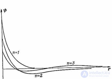
Fig. 5.6. Wave functions of the first three states of the hydrogen atom with l = 0
Example 1. The wave function of the ground state of the electron in the hydrogen atom has the form
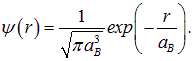
Let us find the probabilities  and
and  of finding the electron inside spheres of radii
  and
and  .
.
The probability of finding the electron in a volume element dV equals

Since the wave function of the ground state does not depend on the direction of the radius vector  , but only on its magnitude r, we can write an expression for the probability
  of finding the electron in a spherical shell of radius r and thickness dr. The volume of this shell equals
  (surface area multiplied by thickness). Then

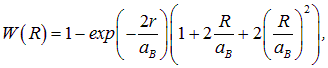
Now we need to integrate the probability over all values of r from 0 to R, obtaining the probability W(R) of finding the electron inside a sphere of radius R:
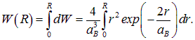
The integral is taken exactly, and as a result we obtain
|
|
|
(5.7) |
from which we find
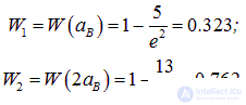
Here e — is the base of the natural logarithm. The difference  gives the probability of finding the electron between the spheres of radii
  and
and  . It can be seen that numerically this probability is close to the probability
  . On the other hand, the probability of finding the electron outside a sphere of radius is noticeably smaller: as is not hard to guess, it equals

In other words, with a probability of more than 76% the electron in the ground state is located at a distance of no more than two Bohr radii from the nucleus.
Example 2. Let us find the electrostatic potential created by the hydrogen atom in the ground state.
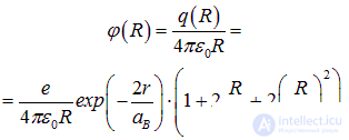
Let us take any point at a distance R from the nucleus. The electrostatic potential at this point is created, firstly, by the positive charge e of the nucleus, and secondly, by that part of the electron's charge which lies inside a sphere of radius R. It is well known that a spherically symmetric charge distribution creates no field in its interior regions. Therefore the part of the electron cloud lying beyond the chosen point makes no contribution to the potential. Since equation (5.7) gives the probability W(R) of finding the electron inside a sphere of radius R, the negative charge inside this sphere equals –eW(R). Therefore the potential at the point R, created by the effective charge

has the form
|
|
|
(5.8) |
At large distances, the potential (5.8) decreases exponentially, that is, much faster than the usual Coulomb potential of a point charge. This is — the so-called screening effect: the negative charge of the electron compensates the positive charge of the nucleus. When

the potential (5.8) turns into the usual Coulomb potential: we have penetrated inside the electron cloud, where it no longer screens the charge of the nucleus.
For the energy, the Schrödinger equation gives exactly the same formula as does Bohr's theory:
|
|
|
(5.9) |
As we can see, the energy indeed does not depend on the quantum numbers l, m. At the same time, as follows from the properties of the solutions of equation (5.6), the azimuthal quantum number l takes integer values from 0 to n – 1. And this property, guessed by us on the basis of classical physics, reproduced itself in quantum mechanics.
It is remarkable how quantum mechanics, having overturned so many classical notions, gives analogous results wherever the symmetry properties of a system come into play. Hence the conclusion: symmetry plays a more important role than specific physical laws. Someday new laws will be discovered that generalize both quantum mechanics and all the theories currently at the forefront of science. But the symmetry properties of the system will manifest themselves one way or another.
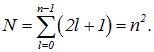
The difference between quantum mechanics and Bohr's theory is a richer structure of states: the state is determined by three quantum numbers, just as in a three-dimensional potential box. Incidentally, this is no accident. The three quantum numbers in the potential well and in the hydrogen atom are a reflection of the three-dimensionality of our space. Let us calculate the degeneracy multiplicity, that is, the number of different states with the same energy (the same principal quantum number n). For a given value of n the number l runs through all integers from 0 to n – 1, and each of them corresponds to 2l + 1 values of n. Therefore the degeneracy multiplicity N is determined by the relation
|
|
|
(5.10) |
At n = 1 we have N = 1, that is, the ground level is not degenerate. At n=2 the degeneracy multiplicity equals 4: one level with l = 0 and three levels with l = 1 and different projections of the angular momentum n = –1, 0, +1. At n = 3 the degeneracy multiplicity N = 9: one level with l = 0, three levels with l = 1 and five levels (by the number of projections) with l = 2. To classify energy states by the value of the quantum number l, conventional notations borrowed from spectroscopy are used, where they appeared even before the theory of the atom was created:
|
l = |
0 |
1 |
2 |
3 |
4 |
5 |
… |
|
symbol |
s |
p |
d |
f |
g |
h |
… |
The principal quantum number is placed in front of the symbol. Examples of possible states:
1s, 2s, 2p, 3s, 3p, 3d, 4s, 4p, 4d, 4f and so on.
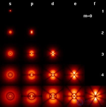
Fig. 5.7. Eigenfunctions of the Hamiltonian for the hydrogen atom. Cross sections of the probability density are shown, its magnitude represented by color (black corresponds to the minimal probability density, and white ̶ to the maximal). Each column corresponds to a definite value of the quantum number l. The principal quantum number n is indicated to the right of each row. For all the pictures the quantum number m = 0. The projection of the angular momentum is taken along the vertical axis z. The cross section is taken in the x, z plane. The probability density in three-dimensional space is obtained by rotating the picture about the z axis
To avoid any misunderstanding, note that the order of states given here is purely «alphabetical». If the states are arranged in order of increasing energy, then in multielectron atoms the list looks different — for example, starting with potassium (Z = 19), the states 3d and 4s swap places. The reasons for such «inversions» are discussed in the corresponding sections further on.
When an electron transitions from a higher energy level to a lower one, it emits a photon carrying away an intrinsic angular momentum equal to ħ (the authors ask you to take this on faith). Consequently, only transitions with a change of l by one are allowed: a selection rule arises
|
When an electron in an atom transitions from one energy level to another, the azimuthal quantum number changes by one
|
This means that in the hydrogen atom the following transitions are allowed

and so on, leading to the same spectral series as in Bohr's theory. The richer structure of states is not yet manifested in a greater variety of atomic levels and, correspondingly, of spectra, because of the degeneracy.
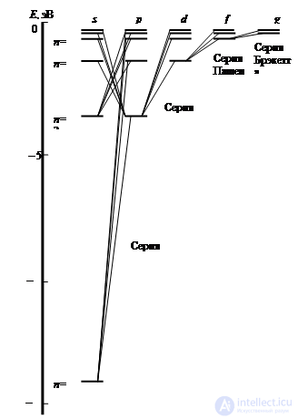
Fig. 5.8. Diagram of the energy levels and possible transitions between levels in the hydrogen atom
Speaking of the degeneracy of levels, we had in mind the hydrogen-like atom. In more complex atoms, or in the presence of external electromagnetic fields, the degeneracy, as they say, is lifted, and a dependence of the energy on the numbers  appears. Any non-Coulomb, centrally symmetric correction to the potential energy leads to a dependence of the energy levels on l (observed, for example, in alkali metals). In classical physics such a correction to the usual law of attraction (say, of a planet to the Sun) turns elliptical orbits into unclosed curves. Moving along such an orbit, a planet, as it were, moves along an ordinary ellipse which additionally rotates as a whole, precessing in the same plane. A similar effect — the precession of Mercury's perihelion — was predicted by general relativity. This new motion leads to an additional rotational energy that depends on l. As a result, the energy of the 2s level ceases to coincide with the energy of the 2pp level, and so on.
Any non-centrally-symmetric field (for example, a magnetic one) lifts the degeneracy in mm. In classical physics a magnetic field causes the plane of rotation to precess about the direction of the field, and this rotation likewise gives rise to additional energy. What has been said can be formulated as a general conclusion:
|
Any additional interaction that breaks the symmetry of a system lifts the corresponding degeneracy of the energy levels. Experimentally, the lifting of degeneracy manifests itself as the splitting of former spectral lines into several components. |
Further study of atomic spectra showed that many spectral lines have two close components. Thus, as early as 1887, A. Michelson discovered the splitting of the  line of the Balmer series in hydrogen, produced by the transition

It turned out to consist of two lines with an average wavelength of 6 563 Å.
|
Ångström (Å) is a non-SI unit of length used in atomic physics 1 Å=10-10mm. |

Fig. 5.9. Albert Abraham Michelson, 1852–1931
The wavelength difference is 0.14 Å (that is, the relative magnitude of the splitting is of order 10–5 ). Lines split into 3, 4 and more components were also found. The splitting of lines, as we now understand, means the splitting of the atom's energy levels: they acquire, as it is said, a fine structure. Hence there is some unaccounted-for interaction. We said that the splitting of lines arises, for example, when an applied external field breaks the symmetry of the system. But here the unaccounted-for interaction manifests itself in the absence of external fields, that is, it must be connected with some internal properties of the atom.
It turned out that this is indeed a manifestation of internal properties, but not of the atom as a whole — of the electron. In 1925 S. Goudsmit and G. Uhlenbeck put forward the hypothesis of electron spin: they proposed that the electron possesses an intrinsic angular momentum, unrelated to its orbital motion. At first spin was imagined as a spinning (English spin) of the electron about its own axis (an analogue of the Earth's daily rotation). Later it was realized that this «spinning» could not be taken literally: numerical estimates gave a linear spinning speed exceeding the speed of light in vacuum.
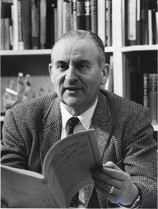
Fig. 5.10. Samuel Abraham Goudsmit, 1902–1978
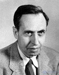
Fig. 5.11. George Eugene Uhlenbeck, 1900–1988
|
Spin is understood as the electron's intrinsic angular momentum, a built-in quantum property of it. |
Its existence remains a mystery if one stays only within the framework of Heisenberg–Schrödinger quantum mechanics. Spin received a natural explanation only in P. Dirac's relativistic quantum theory, which united relativity with quantum mechanics.
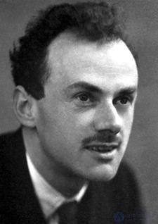
Fig. 5.12. Paul Adrien Maurice Dirac, 1902–1984
Experiments showed that the electron must be assigned a spin quantum number s = 1/2, which has the same properties (see formula (5.5)) as the quantum number l. For brevity, the spin quantum number is customarily called simply the spin. We too will use this generally accepted terminology from now on.
Accordingly, there exists a single eigenvalue of the operator of the
продолжение следует...
Часть 1 5. The theory of the atom
Часть 2 5.6. The Pauli Principle and the Valence of Elements -
Часть 3 - 5. The theory of the atom
 and
and  have a common set of eigenstates if and only if they commute:
 and
and  do not commute, the coordinate of a particle and the projection of its momentum onto the same axis cannot be measured exactly and simultaneously.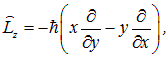
 does not contain the angle
  itself, but only the derivative with respect to it. This means that the operator
  .
. and
and  ).
). can take only integer values in units of Planck's constant
 ;
; ;
;



Comments