
Lecture
|
Oscillations — are physical processes characterized by some degree of repeatability. |
Depending on the physical nature of the repeating process, oscillations are distinguished as: mechanical, electromagnetic, electromechanical, etc.
Depending on the nature of the influence on the oscillating body, a distinction is made between free (or natural) and forced oscillations.
If the position of a system at any time can be described by a single parameter, then the system has one degree of freedom. Examples of such systems: a pendulum oscillating in a given plane; a mass attached to a spring; an LC-circuit (Fig. 1.1). Such systems are usually given the general name oscillator (from the English oscillate — to oscillate, vibrate).

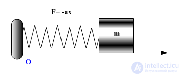
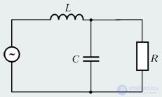
Fig. 1.1. Examples of oscillatory systems with one degree of freedom.
In this section we will show that the equations of oscillatory motion of many systems are, in essence, the same, so that different physical processes can be described by one and the same mathematical formulas.
Spring pendulum
|
Spring pendulum — is a system consisting of a ball of mass m, suspended on a spring of length |
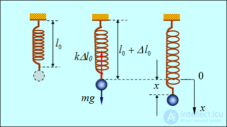
Fig. 1.2. Toward the derivation of the equation of motion for a spring pendulum
In the equilibrium position (Fig. 1.2) the force of gravity  is balanced by the elastic force
  :
:

from which
|
|
|
(1.1) |
where  – is the static elongation of the spring. Let us direct the axis x downward and choose the origin such that the coordinate x = 0 corresponds to the position of the ball at rest in the equilibrium position.
If now the ball is pulled away from the equilibrium position by a distance x, then the total elongation of the spring becomes equal to  . By Hooke's law, the projection of the resultant force on the axis OX will then be equal to
|
|
|
(1.2) |
Taking into account that

we obtain
|
|
|
(1.3) |
The minus sign means that the force tends to reduce the deviation from the equilibrium position. The expression obtained corresponds to the elastic force of a weakly deformed spring.
Let us now write the equation of Newton's second law:

It can also be represented in the form:
|
|
|
(1.4) |
|
|
|
|
Video 1.1 Weights on springs. Dependence of the oscillation frequency on the mass of the weight and the stiffness of the spring
Mathematical pendulum
|
Mathematical pendulum — is an idealized system consisting of a weightless and inextensible string, on which is suspended a mass concentrated at a single point. |
We shall characterize the deviation of the pendulum from the equilibrium position by the angle  , which the string makes with the vertical (Fig. 1.3).
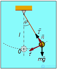
Fig. 1.3. Toward the derivation of the equation of motion of a mathematical pendulum
When the pendulum deviates from the equilibrium position, the material point of mass m is acted on by the force of gravity  and the tension force of the string
  . Accordingly, the equation of motion of this material point has the form
 .
.
Projecting it onto the directions of the normal and the tangent to the trajectory (a circle of radius  ), we obtain
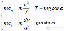
The magnitude of the velocity  is equal to
  ; taking into account that as the point moves toward the equilibrium position the angle decreases, while the speed of the point increases, we write
 .
.
Then the second of the equations of motion written above takes the form
|
|
|
(1.5) |
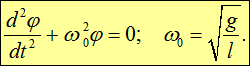
For small deviations of the pendulum from the vertical, when  ,
,

we obtain:
|
|
|
(1.6) |
Physical pendulum
|
Physical pendulum — is an extended oscillating body fixed on an axis. Its dimensions are such that it cannot be considered as a material point. |
An example of a physical pendulum is shown in Fig. 1.4.
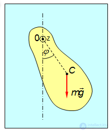
Fig. 1.4. Toward the derivation of the equation of motion of a physical pendulum
When the pendulum deviates from the equilibrium position by an angle  a torque arises tending to return the pendulum to the equilibrium position. This torque is equal to
|
|
|
(1.7) |
where m – is the mass of the pendulum, and l – is the distance 0C between the suspension point 0 and the center of mass Cof the pendulum.

Regarding as a vector associated with the direction of rotation by the right-hand screw rule, the opposite signs of  and can be explained by the fact that the vectors
  and
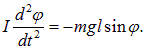
and  are directed in opposite directions. Denoting the moment of inertia of the pendulum about the axis passing through the suspension point as I, we can write the basic equation of the dynamics of rotational motion for the pendulum:
|
|
|
(1.8) |
Let us restrict ourselves to considering small deviations from the equilibrium position:

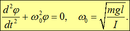
In this case, the equation of oscillation takes the form:
|
|
|
(1.9) |
In the case where a physical pendulum can be represented as a material point oscillating on a string of length l, the moment of inertia is equal to

and we arrive at equation (1.6) for the motion of the mathematical pendulum.
Oscillations of a piston in a vessel with an ideal gas
Let us consider a cylinder with cross-sectional area  , into which is inserted a piston of mass
  (Fig. 1.5). Below the piston in the cylinder is an ideal gas with adiabatic index
  , above the piston is air at constant (atmospheric) pressure
  . The piston can move up and down in the cylinder without friction. We shall assume that in equilibrium the volume of the ideal gas under the piston is equal to
  and that the changes in gas volume caused by the motion of the piston occur adiabatically, that is, without heat exchange with the walls of the cylinder and the piston.
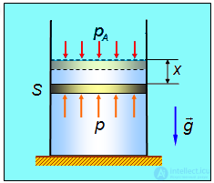
Fig. 1.5. Oscillations of a piston closing a vessel with an ideal gas
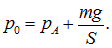
In the equilibrium state, the pressure in the gas under the piston is made up of the atmospheric pressure  and the pressure
  , exerted by the piston. Let us denote this resultant pressure
  :
:
|
|
|
(1.10) |
Let us move the piston a distance x upward. The volume of the vessel will increase and become equal to

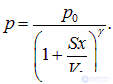
The pressure will decrease accordingly. Assuming there is no heat exchange, the new pressure in the gas can be found from the Poisson adiabatic equation

whence
|
|
|
(1.11) |
Here  is the adiabatic index, which depends on the number of degrees of freedom of the gas molecules.
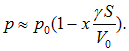
For small oscillations, when the change in gas volume  is much smaller than its «equilibrium» value
  , that is, when

expression (1.11) can be expanded in a Taylor series:
|
|
|
(1.12) |
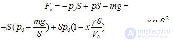
Three forces act on the piston: the force of atmospheric pressure  , the force of gas pressure beneath the piston
  and the force of gravity
  . The signs of the forces correspond to the choice of the positive direction of the x axis upward. Using (1.10) and (1.12), we find for the resultant
  of these forces:
|
|
|
(1.13) |
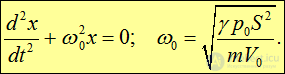
Using (1.13), the equation of motion of the piston

can be written in the following form
|
|
|
(1.14) |
Electromagnetic circuit
Let us consider an oscillatory circuit consisting of a capacitor of capacitance C and a coil of inductance L (Fig. 1.6).
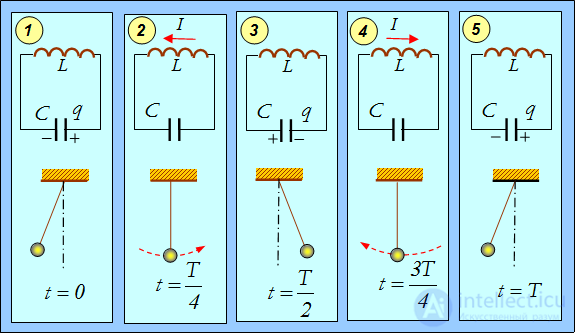
Fig. 1.6. Electromagnetic oscillatory circuit: 1 – t = 0; 2 – t = T/4; 3 – t = T/2; 4 – t = 3T/4; 5 – t = T
We neglect the resistance of the coil and wires. Suppose a current I flows in the circuit, charging the capacitor:

Since no external emf is applied to the circuit, the self-induction emf

is equal to the voltage q/C across the capacitor.
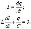
We have two equations:
|
|
|
(1.15) |
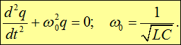
Substituting the first equation into the second, we obtain the equation for the change of charge on the capacitor:
|
|
|
(1.16) |
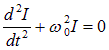
Instead of the substitution used, expressing the current in terms of the charge, we can differentiate the second of equations (1.15) and express the derivative of the charge in terms of the current. As a result, we obtain a similar equation for the change of current in the circuit:
|
|
|
(1.17) |
with the same expression for  , as in (1.16).
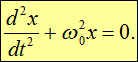
We have considered several physically completely different systems, and we have seen that the equations of motion reduce to the same form
|
|
|
(1.18) |
The differences between the physical systems appear only in the different definition of the quantity  and in the different physical meaning of the variable x: it may be a coordinate, an angle, a charge, a current, etc. Note that, as follows from the very structure of equation (1.18), the quantity always has the dimension of inverse time.
Equation (1.18) describes what are called harmonic oscillations.
|
Harmonic oscillations — are oscillatory motions in which the displacement of the body from the equilibrium position occurs according to a sine or cosine law. |
The equation of harmonic oscillations (1.18) is a linear second-order differential equation (since it contains the second derivative of the variable x). The linearity of the equation means that
It has also been proven mathematically that a second-order equation has two independent solutions. All other solutions, by the properties of linearity, can be obtained as linear combinations of them. By direct differentiation it is easy to check that the independent functions  and
and  satisfy equation (1.18). Hence, the general solution of this equation has the form:
|
|
|
(1.19) |
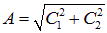
where C1, C2 — arbitrary constants. This solution can also be represented in another form. Let us introduce the quantity
|
|
|
(1.20) |
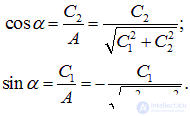
and define the angle  by the relations:
|
|
|
(1.21) |
Then the general solution (1.19) is written as
|
|
|
(1.22) |
According to the formulas of trigonometry, the expression in brackets is equal to

Finally, we arrive at the general solution of the equation of harmonic oscillations in the form:
|
|
|
(1.23) |
The non-negative quantity A is called the amplitude of the oscillation, — the initial phase of the oscillation. The whole argument of the cosine — the combination  — is called the phase of the oscillation.
Expressions (1.19) and (1.23) are completely equivalent, so we can use either of them, depending on considerations of simplicity. Both solutions are periodic functions of time. Indeed, sine and cosine are periodic with period  . Therefore, the various states of a system undergoing harmonic oscillations repeat after a time interval t*, over which the phase of oscillation acquires an increment that is a multiple of :
|
|
|
(1.24) |
It follows that

The smallest of these times
|
|
|
(1.25) |
is called the period of oscillation (Fig. 1.8), and  — its circular (cyclic) frequency.
Fig. 1.8.
The frequency of oscillation is also used
|
|
|
(1.26) |
|
Frequency of oscillation |
Accordingly, the circular frequency is equal to the number of oscillations in seconds.
|
In the SI system, the unit of measurement of frequency is inverse seconds, for which a special name has been introduced — hertz (1 Hz=1/s). |
So, if the system at time t is characterized by the value of the variable x(t), then the variable  will have the same value after a time interval
  (Fig. 1.9), that is
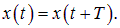
This same value will naturally repeat after a time 2T, 3T and so on.
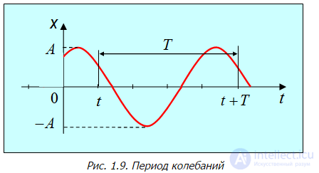
Fig. 1.9. Period of oscillation
The general solution includes two arbitrary constants (C1, C2 or A, a), whose values must be determined by two initial conditions. Usually (although not necessarily) their role is played by the initial values of the variable x(0) and its derivative  .
.
Let us give an example. Suppose the solution (1.19) of the harmonic oscillation equation describes the motion of a spring pendulum. The values of the arbitrary constants depend on the way in which we displaced the pendulum from the equilibrium state. For example, we pulled the spring back a distance  and released the ball with no initial velocity. In this case
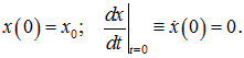
Substituting t = 0 into (1.19), we find the value of the constant C2
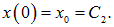
The solution thus has the form:

We find the velocity of the mass by differentiating with respect to time

Substituting here t = 0, we find the constant C1:
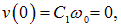
whence

Finally
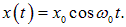
Comparing with (1.23), we find that  is the amplitude of oscillation, and its initial phase equals zero:
  .
.
Let us now displace the pendulum from equilibrium in a different way. We strike the mass so that it acquires an initial velocity  , but is practically not displaced during the impact. We then have different initial conditions:
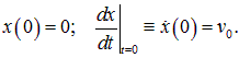
Since
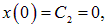
our solution has the form
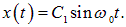
The velocity of the mass will change according to the law:
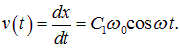
Let us substitute here  :
:
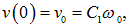
whence

Finally we obtain:
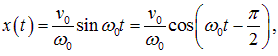
so that the amplitude of oscillation is equal to

and the initial phase

In the general case, when the initial displacement of the pendulum from the equilibrium position is  , and the initial velocity is , the relation of these quantities to the amplitude and initial phase of oscillation has the form
|
|
|
(1.27) |
Differentiating solution (1.22) with respect to time, we find the time dependence of the velocity and acceleration of the pendulum:
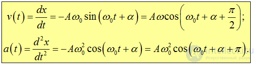
The corresponding graphs are shown in Fig. 1.10 (for simplicity we have set the initial phase  ). It can be seen that the velocity and acceleration also change according to a harmonic law, with the amplitude of the velocity being
  , and the amplitude of the acceleration
  . The velocity leads the displacement in phase by
  , while the acceleration is in antiphase with respect to the displacement. This means that at the moment when the displacement reaches its greatest positive value, the acceleration reaches its greatest negative value in magnitude, and vice versa.
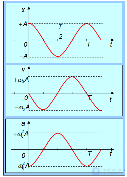
Fig. 1.10. Time dependence of the position, velocity and acceleration of an oscillating material point
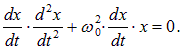
Let us multiply the harmonic oscillation equation (1.18) by the rate of change of the variable x:
|
|
|
(1.28) |
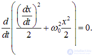
Each of the terms can be represented as the corresponding derivative:
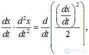
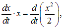
so that equation (1.28) is written in the form:
|
|
|
(1.29) |
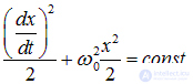
It follows that the quantity in brackets does not depend on time, that is, it is conserved during the oscillation process:
|
|
|
(1.30) |
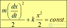
To clarify the physical meaning of the conserved quantity, let us apply these relations to the spring pendulum, for which

We see that equation (1.30) can be written as the sum of the kinetic energy of the mass and the potential energy of the deformed (compressed or stretched) spring:
|
|
|
(1.31) |
Thus, the conservation law we have found is none other than the law of conservation of total energy of the system.
Similarly, for the electromagnetic circuit the variable
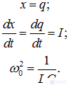
and

In this case relation (1.30) takes the form:
|
|
|
(1.32) |
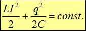
The first term is the energy of the magnetic field in the coil, and the second is the energy of the electric field in the capacitor. Again we have obtained that the total energy of the system is conserved.
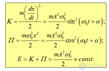
Returning to the general form (1.30) of the energy conservation law and substituting into it the general solution (1.23), we obtain the laws of change with time of the kinetic and potential energies (or their analogues) and an expression for the conserved total energy:
|
|
|
(1.33) |
It follows that
Video 1.9 Conservation of energy in near-harmonic oscillations – Galileo's pendulum.
What has been said is illustrated in Fig. 1.11, which shows the changes in kinetic and potential energy for a spring pendulum and an electromagnetic circuit.
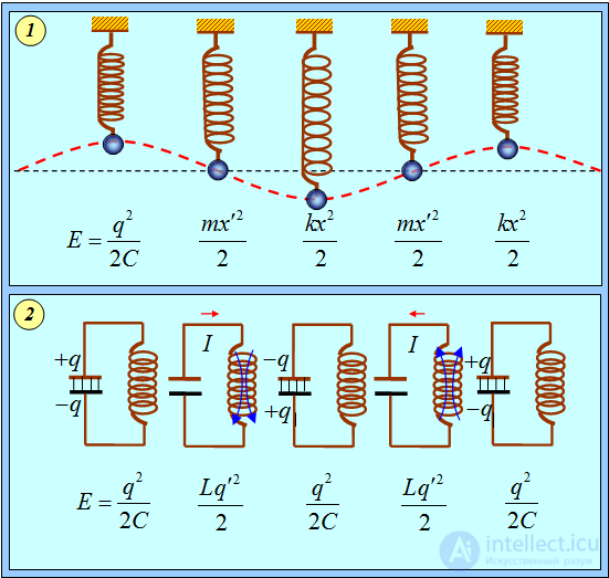
Fig. 1.11. Changes with time of various forms of energy in an oscillatory system:
1 – spring pendulum; 2 – electromagnetic oscillatory circuit
It may happen that an oscillator takes part in two oscillations of the same direction with different amplitudes, frequencies and initial phases. Let us consider the addition of such oscillations.
Addition of oscillations with equal frequencies
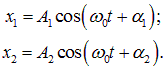
For simplicity, let us first consider the case in which the frequencies of the oscillations being added are equal. The general solutions of the harmonic oscillations being added have the form:
|
|
|
(1.34) |
where x1, x2 — variables describing the oscillations, A1, A2 — their amplitudes, and  ,
,  — the initial phases. The resulting oscillation

is conveniently found using a vector diagram. This method uses the analogy between rotation and the oscillatory process.
Let us take the general solution (1.23) for a harmonic oscillation. Let us choose the axis 0x. From the point 0 let us lay off a vector of length A, forming with the axis 0x the angle  . If this vector is set into rotation with angular velocity
  , then the projection of the end of this vector will move along the axis 0x from +A to –A, with the value of the projection changing according to the law
|
|
|
(1.35) |
Thus, the projection of the end of the vector onto the axis 0x will perform harmonic oscillations with an amplitude equal to the length of the vector, with a circular frequency equal to the angular velocity of rotation of the vector, and with an initial phase equal to the angle formed by the vector with the axis at the initial moment of time (Fig. 1.12).
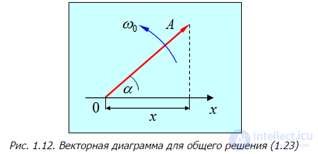
Fig. 1.12. Vector diagram for the general solution (1.23)
Let us now apply this technique to the addition of oscillations (1.34). Let us represent both oscillations by means of the vectors A1 and A2 Let us take their vector sum (Fig. 1.13)

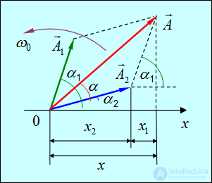
Fig. 1.13. Vector diagram for the addition of equally directed oscillations of the same frequency
The projection of the vector A1 onto the axis 0x equals the sum of the projections of the corresponding vectors

Thus, the vector A represents the resulting oscillation. This vector rotates with the same angular velocity  , so that the resulting motion will be a harmonic oscillation with frequency
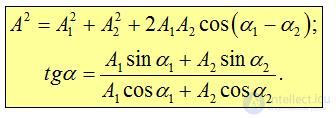
  , amplitude A and initial phase a. According to the law of cosines:
|
|
|
(1.36) |
In particular, if the phases of the oscillations being added are equal or differ by a value that is a multiple of  (that is
 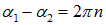 ), then the amplitude of the resulting oscillation equals the sum of the amplitudes

If, on the other hand, the oscillations being added are in antiphase (that is  ), then

Beats
In this section we shall consider the case of adding equally directed harmonic oscillations with different frequencies. In practice, of particular interest is the case where the oscillations being added differ little in frequency. As we shall see, the addition of these oscillations results in oscillations with a periodically varying amplitude, called beats.
|
Beats — this is the periodic variation of the amplitude of oscillations that arises when two harmonic oscillations of close frequencies are added. |
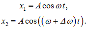
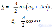
For simplicity let us consider the case where the amplitudes of the oscillations being added are equal to A, and the initial phases of both oscillations are equal to zero. The frequencies of the oscillations being added are, respectively,  and
and  . So,
. So,
|
|
|
(1.37) |
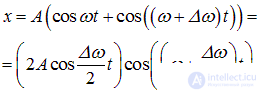
Let us add these expressions and take into account the well-known trigonometric formula:
|
|
|
(1.38) |
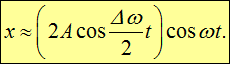
If  then in the argument of the second cosine we can neglect the frequency shift:
|
|
|
(1.39) |
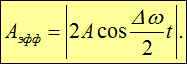
In addition, the factor in brackets changes slowly compared with  . Therefore the resulting oscillation x can be regarded as a modulated harmonic oscillation with frequency w, whose effective amplitude
  changes with time according to law (1.40) (Fig. 1.14):
|
|
|
(1.40) |
Let us emphasize that, strictly speaking, such an oscillation is not harmonic, and let us once again recall that, by definition, an oscillation is harmonic if it occurs according to the law 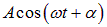 , with all three of its parameters:
  being strictly constant in time.
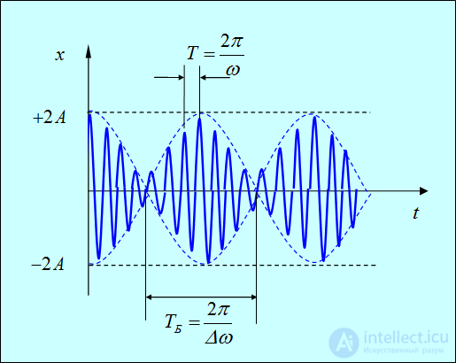
Fig. 1.14. Beats arising from the addition of oscillations with close frequencies
The frequency of amplitude pulsation (called the beat frequency) equals the difference of the frequencies of the oscillations being added. The beat period is equal to
|
|
|
(1.41) |
Video 1.12 Beats on an oscilloscope screen
Video 1.13 Beats: oscilloscope and speaker
Video 1.14 «Double» pendulum: recording the pattern of beats in sand
Oscillations of two coupled oscillators
Let us give an instructive example of a system in which beats arise. Consider two masses of mass m, which can oscillate under the action of two identical springs with stiffness coefficients k. Let the masses also be connected by a soft spring with stiffness coefficient K<. We shall assume the unstretched lengths of all the springs to be equal, namely 2L (Fig. 1.15).
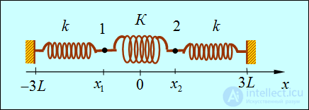
Fig. 1.15. An example of coupled oscillators.
The oscillations occur along the 0x axis; gravity is not taken into account
Then in the equilibrium position the coordinates of the masses are equal to

During oscillation the coordinates are, respectively, equal to x1(t), x2(t). The elongations of the springs are written as
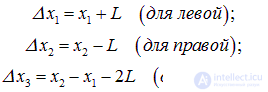
We are dealing with a system having two degrees of freedom. Let us set up the equations of motion. The first mass is acted upon by a force from the spring k, equal to
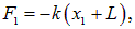
and a force from the spring K, equal to

The second mass is acted upon by similar forces
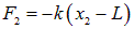
and

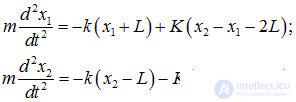
Accordingly, the equations of motion have the form
|
|
|
(1.42) |
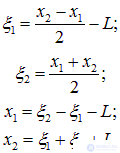
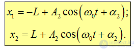
At first glance these equations do not look very much like the equations of harmonic oscillations, because the oscillations x1 are influenced by the oscillations x2 and vice versa. Let us therefore transform the equations to new variables, for which the equations would be independent (such variables are called normal coordinates, and the corresponding oscillations — normal oscillations (modes)). Namely, let us introduce new variables x1 and x2:
|
|
|
(1.43) |
As is easy to verify, the equilibrium positions correspond to zero values of these coordinates
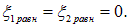
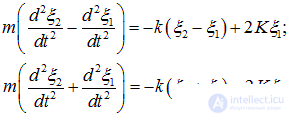
In these variables equations (1.42) take the form:
|
|
|
(1.44) |
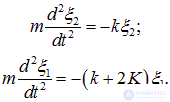
Adding and subtracting these equations, we arrive at a pair of independent equations for the introduced normal coordinates:
|
|
|
(1.45) |
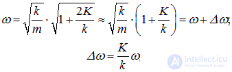
The first equation describes harmonic oscillations with frequency

coinciding with the frequency of oscillation of the spring pendulums in the absence of the connecting spring K. The second equation describes oscillations with a shifted frequency
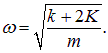
Since K<, we have
|
|
|
(1.46) |
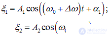
Accordingly, we obtain the general solution of the system of equations:
|
|
|
(1.47) |
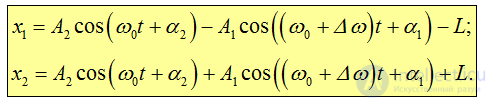
The general solution for the coordinates x1 and x2 of the oscillating points follows from (1.47) and (1.43):
|
|
|
(1.48) |
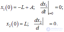
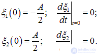
As an example, let us consider the case when the first mass is displaced a distance  from the equilibrium position and released with zero initial velocity, while the second mass remains at the equilibrium position:
|
|
|
(1.49) |
These correspond to the following initial values of the normal coordinates:
|
|
|
(1.50) |
Such initial conditions have already been considered above. The corresponding solutions have the form
|
|
|
(1.51) |
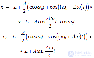
Substituting the amplitudes and initial phases found into (1.48), we obtain the solutions describing the oscillations of the masses under consideration about their equilibrium positions:
|
|
|
(1.52) |
Graphs of the functions x1(t), x2(t) are shown in Fig. 1.16. The characteristic pattern of beats is visible.
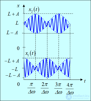
Fig. 1.16. Beats in a system of two coupled oscillators
At the initial moment of time only the first mass oscillates. Then the second begins to oscillate, while the amplitude of oscillation of the first decreases. After a time  the first mass stops, while the second oscillates with the maximum possible amplitude. A «transfer» of energy from the first pendulum to the second has occurred. Then the process of energy «transfer» proceeds in the opposite direction, and by the moment
  the first pendulum oscillates with maximum amplitude, while the second is at rest.
Fig. 1.17 demonstrates beats in a system of two coupled mathematical pendulums.
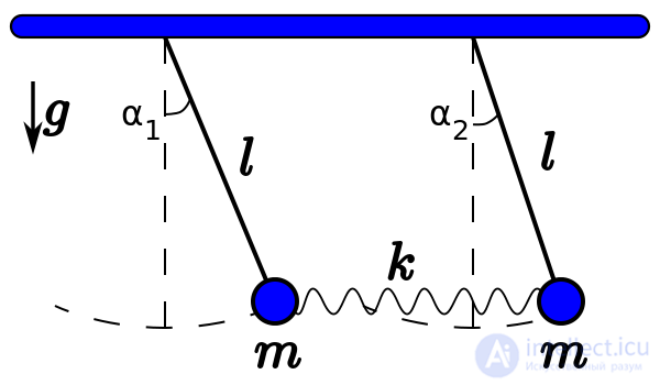
Fig. 1.17. Beats in a system of coupled pendulums
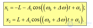
Let us now clarify the physical meaning of the normal modes corresponding to purely harmonic oscillations of the system. If only the first of them (x1) is excited, then A2 = 0 and, as follows from the general solution (1.48),
|
|
|
(1.53) |
From (1.53) it is seen that the first normal mode corresponds to an oscillation in which both masses are displaced by equal distances from their equilibrium positions, but in opposite directions; in other words — they oscillate in antiphase. The velocities of the masses are also equal in magnitude and opposite in direction, so that the center of mass of the masses remains stationary. The oscillations occur under the action of the springs of stiffness k, to which is added the connecting spring of stiffness K. As a consequence, the frequency of such oscillations is greater than the frequency of oscillation of the uncoupled oscillators
Excitation of only the second (x2) normal mode means that A1 = 0:
|
|
|
(1.54) |
In this case the masses are displaced from the equilibrium position in the same direction by equal distances; in other words – they oscillate in phase. Their velocities are likewise equal in magnitude and direction. The connecting spring oscillates together with the masses, but remains unstretched and therefore has no effect, so that the frequency of oscillation coincides with the frequency of oscillation of the uncoupled pendulums.
In the case analyzed we have become acquainted with normal modes and found that their frequencies are shifted compared with the frequencies of oscillation of the uncoupled pendulums. Any other oscillatory motion of the system can be represented as a superposition of normal modes. In a similar way one can consider a chain of many oscillators coupled to one another and study their normal oscillations. Such a system represents a model of a crystal lattice.
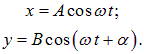
In this section we shall consider the addition of two harmonic oscillations of the same frequency  , occurring in mutually perpendicular directions along the axes x and y. Let us choose the origin of time so that the initial phase of the first oscillation is equal to zero:
|
|
|
(1.55) |
where  is the phase difference between the two oscillations. Let us find the equation of the trajectory of the oscillating material point, that is, the function
  .
.
Let us first consider particular cases. Let the phase difference be equal to zero:  . Then
|
|
|
(1.56) |
that is, the trajectory of the point is a straight line. A similar trajectory is obtained for oscillations with phase difference 
|
|
|
(1.57) |
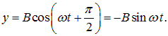
For phase difference  we find:
|
|
|
(1.58) |
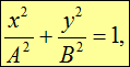
From (1.58) and (1.55) follows the equation of an ellipse:
|
|
|
(1.59) |
with the point moving clockwise (for the standard orientation of the axes: the OX axis — to the right, the OY axis — upward). For phase difference  we find:
|
|
|
(1.60) |
This leads to the same elliptical trajectory (1.59), except that in this case the rotation is counterclockwise.
If the oscillation amplitudes along the x and y axes are equal ( ), then a circular trajectory is obtained from (1.59).
In the general case of an arbitrary phase difference  the trajectory will also be an ellipse, but with rotated axes (Fig. 1.18).
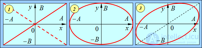
Fig. 1.18. Trajectories of a material point oscillating with equal frequencies
in mutually perpendicular directions, for various phase differences:
1 —  or
or  (dashed line); 3 —
  ; 2 —
; 2 — 
Video 1.15 Airy pendulum: sand recording of Lissajous figures
Video 1.16 Lissajous figures on an oscilloscope screen
If the frequencies of the mutually perpendicular oscillations are not equal, the trajectory of the resulting motion has a rather complex shape. Closed trajectories described by a point undergoing two mutually perpendicular oscillations simultaneously arise when the ratio of the frequencies of the added oscillations is a rational number; such trajectories are called Lissajous figures.
One of the simplest Lissajous figures is obtained for a frequency ratio of 2:1 and zero initial phases  :
:
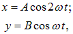
whence
|
|
|
(1.61) |
We have obtained the equation of a parabola.
The shape of the Lissajous figures depends on the ratio of the frequencies of the added oscillations and the phase difference between them. Examples of adding oscillations with various frequency ratios are shown in Fig. 1.19 and 1.20.
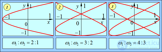
Fig. 1.19. Examples of Lissajous figures for the indicated frequency ratios and zero values of the initial phases of each oscillation.
The coordinate x is expressed in units of the amplitude A, and the coordinate y – in units of the amplitude B.
The frequency  refers to the oscillations along the x axis,
  – along the y
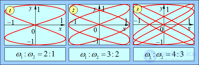
Fig. 1.20. Examples of Lissajous figures for the same frequency ratios as in Fig. 1.19 and the same initial phases of each oscillation 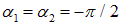 , that is, for

Harmonic oscillations existing forever are one of the physical abstractions. In real systems, oscillations die out after some time due to energy dissipation. Thus, the concept of harmonic oscillations can only be used for times small compared to the characteristic damping time. Damping of oscillations will always be observed in systems with friction.
The equation of damped oscillations
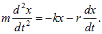
Let us consider, as an example, a spring pendulum placed in a viscous medium. In addition to the elastic force, a resistance force proportional to the velocity will act on the body

where r — is the corresponding coefficient, depending on the viscosity of the medium and the size and shape of the body. Therefore the equation of motion takes the form:
|
|
|
(1.62) |
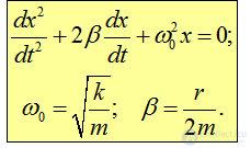
or
|
|
|
(1.63) |
Here  is a new, additional parameter of the system, called the damping coefficient. The oscillations are undamped if
  .
.
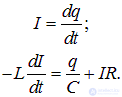
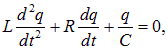
Another example — an electromagnetic circuit. If, besides the capacitor C and inductance L the circuit also has active resistance R, then the self-induction emf equals the sum of the voltage across the capacitor and the voltage drop across the resistance. Therefore equations (1.15) now take the form:
|
|
|
(1.64) |
Substituting the first equation into the second:
|
|
|
(1.65) |
or
|
|
|
(1.66) |
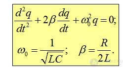
Recall that the combination L/R has already appeared in the theory of electromagnetism, where it characterized the characteristic time of decay (appearance) of extra currents at closing-opening. Thus, the quantity b has the dimension of inverse time, coinciding with the dimension of angular frequency.
Analysis of the solutions
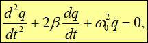
Thus, in both cases considered, the differential equation of free damped oscillations of a linear system has the form:
|
|
|
(1.67) |
|
|
|
|
 — the damping coefficient, and
  — the angular frequency of free (natural) undamped oscillations (that is, at
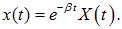
  , in the absence of energy losses). Let us reduce the new problem to the previous one. To do this, instead of the variable x we define a new variable X, related to x by the relation:
|
|
|
(1.68) |
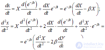
Differentiating the function x(t), we obtain:
|
|
|
(1.69) |
Substituting these expressions into (1.67):
|
|
|
(1.70) |
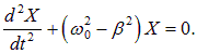
The expression in square brackets must equal zero. We note that in this expression the terms with the first derivative  cancel. As a result we obtain the differential equation for the function X(t):
|
|
|
(1.71) |
Two cases are possible here. Suppose first that  . Then we can introduce the parameter
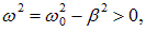
so that equation (1.71) takes the form:
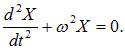
But this is — the standard equation of harmonic oscillations, whose general solution we know:

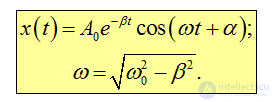
Thus, we have found the general solution of the equation of damped oscillations (1.67):
|
|
|
(1.72) |
In many systems the damping coefficient is small compared to the natural frequency of oscillation:  . Then the motion of the system can be regarded as an almost harmonic oscillation with frequency
  and with an amplitude changing according to the law (Fig. 1.22)

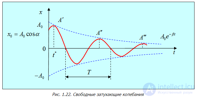
Fig. 1.22. Free damped oscillations
Video 1.17 Mechanical (pendulum) damped oscillations — sand recording
Video 1.18 Damping of tuning fork oscillations — oscilloscope and one's own ears
The damping coefficient  determines the rate of decrease of the oscillation amplitude: it is the inverse of the time interval over which the amplitude decreases by a factor of e.
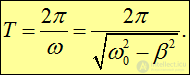
The period of damped oscillations equals:
|
|
|
(1.73) |
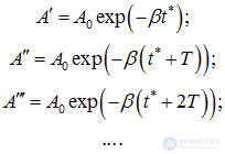
Let the first largest positive deviation be reached at time  . The subsequent largest deviations of the same sign (A', A'', A''' etc. — see Fig. 1.22) form a geometric progression:
|
|
|
(1.74) |
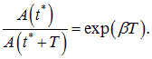
The ratio of the amplitude values corresponding to times differing by one period equals:
|
|
|
(1.75) |
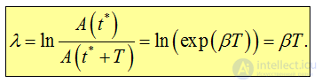
This ratio is called the damping decrement. The logarithm of this ratio is called the logarithmic damping decrement:
|
|
|
(1.76) |
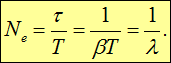
Let us determine the number of oscillations the system performs over the time  . Over this time the amplitude decreases by a factor of e, and the number of oscillations equals:
|
|
|
(1.77) |
Consequently, the logarithmic damping decrement is the inverse of the number of oscillations performed during the time over which the amplitude decreases by a factor of e.
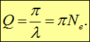
To characterize an oscillatory system, a quantity called the quality factor:
|
|
|
(1.78) |
is often used, which is proportional to the number of oscillations Ne, performed by the system over the time  , during which the oscillation amplitude decreases by a factor of e. For example, for an electromagnetic circuit at
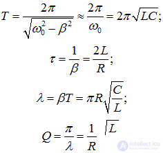
  we find:
|
|
|
(1.79) |
We have seen that the total energy in an oscillating system is proportional to the square of the amplitude. For small damping ( ) we have:
|
|
|
(1.80) |
where E0 — is the value of the total energy of the oscillating system at the initial moment of time. We can determine the energy loss over a period T:
|
|
|
(1.81) |
Consequently,
|
|
|
(1.82) |
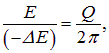
that is, for weak damping the quality factor, up to a factor of  , equals the ratio of the total energy stored in the oscillatory system at a given moment of time to the energy loss over one period of oscillation.
As the damping increases, the oscillation frequency
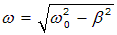
tends to zero, and the period of oscillation grows. In the limiting case

the period becomes infinite, that is, the motion ceases to be periodic. The corresponding mathematical analysis shows that for  the motion is aperiodic in character — the system, displaced from its equilibrium position, returns to the equilibrium position without oscillating.
In the case of forced oscillations, the system oscillates under the action of a periodic external (driving) force. The energy losses of the system are compensated by the work of this force. The frequency of the forced oscillations depends on the frequency of variation of the external force (for brevity we will call it the "driving frequency"). Of the greatest practical interest is the case where the driving force varies according to a harmonic law:

The dependence of the amplitude of the forced oscillations on the frequency of the driving force leads to the fact that at a certain frequency, specific to a given system, the oscillation amplitude reaches a maximum value. This phenomenon is called resonance.
|
Resonance — is the phenomenon of a sharp increase in the amplitude of forced oscillations at a certain frequency of external action, called the resonant frequency of the system. |
Video 1.21 Resonant interaction of pendulums
Video 1.22 Tuning forks: resonant absorption of wave energy
Video 1.23 Resonance of a board with a motor
The phenomenon of resonance is used to amplify oscillations, for example electrical ones. However, when designing machines and structures, the phenomenon of resonance must be taken into account in order to prevent the most often undesirable, and sometimes destructive, consequences of a resonant increase in the amplitude of forced oscillations.
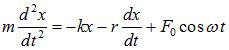
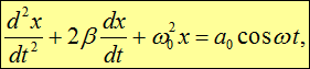
For a spring pendulum, the equation of forced oscillatory motion has the form:
|
|
|
(1.83) |
or
|
|
|
(1.84) |
where
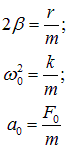
and  — is the driving frequency.
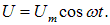
If we consider an electric oscillatory circuit, the energy losses in the circuit can be compensated by means of an externally applied emf or alternating voltage, periodically varying according to a harmonic law
|
|
|
(1.85) |
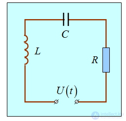
Fig. 1.25. Forced oscillations in an electromagnetic circuit
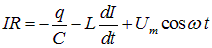
The equation of oscillations in the circuit (Fig. 1.25) can be written using Ohm's law for a closed circuit
|
|
|
(1.86) |
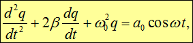
or, taking into account that 
|
|
|
(1.87) |
where

— the natural frequency of the circuit,

— the damping coefficient, and

Thus, forced oscillations in an electric circuit are described by the same linear inhomogeneous second-order differential equation as in the case of oscillations of a spring pendulum. Suppose we know at least one solution of this equation — some particular solution  . Then the difference between any other solution q(t) and this particular solution
  will satisfy the homogeneous equation (with zero on the right-hand side), which we studied in detail in the previous section. Therefore the general solution of equation (1.87) can be written as
|
|
|
(1.88) |
where
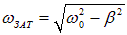
— the frequency of free damped oscillations.
With time, due to the exponential factor  the role of the second term decreases (it is important at the initial stage of establishment of the oscillations). After a sufficiently long time, namely, at
 ,
,
it can be neglected, keeping only the first term. Thus, the problem of studying the steady-state forced oscillations reduces to finding at least one particular solution of equation (1.87).
We will seek the particular solution of the inhomogeneous equation in the form of a harmonic function whose frequency of variation coincides with the frequency of the driving force:
|
|
|
(1.89) |
Substitute  in the form (1.89) into equation (1.87):
|
|
|
(1.90) |
Since the sine and cosine functions are linearly independent, the coefficients before them on the left-hand side of (1.90) must equal zero:
|
|
|
(1.91) |
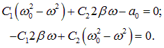
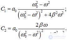
The solution of this system has the form:
|
|
|
(1.92) |
The solution (1.89) with coefficients (1.92) can be written in the standard form:
|
|
|
(1.93) |
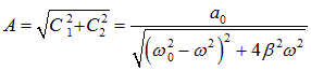
where
|
|
|
(1.94) |
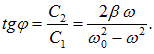
and
|
|
|
(1.95) |
With the minus sign in the phase of the cosine in expression (1.93), the initial phase  has a simple physical meaning: it is the lag in phase of the steady-state forced oscillation behind the harmonic driving «force» (1.85).
Video 1.24 Resonant reed frequency meter
Video 1.25 Spectrum of a modulated oscillation
Let us consider the response of the system to a change in the frequency of the external force. Under the square root in the expression for the amplitude is a quadratic function of frequency

This function has a minimum (and hence the amplitude has a maximum).
To find the minimum point we differentiate the function  with respect to
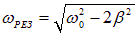
  and set the derivative equal to zero. As a result we obtain the following expressions for the resonant frequency
|
|
|
(1.96) |
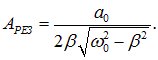
and the amplitude of the steady-state forced oscillations at resonance
|
|
|
(1.97) |
It should be noted that for  the value of the resonant frequency
  practically coincides with the natural frequency
  of the oscillatory system. Since
  appears in the denominator of the expression for
  , the resonant amplitude of the oscillations grows as the damping decreases. Graph 1.26 shows that the smaller the damping, the higher and further to the right lies the maximum of the resonance curve.
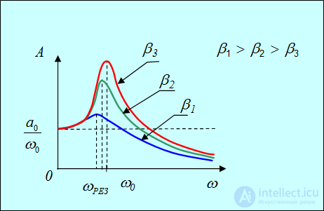
Fig. 1.26. Dependence of the amplitude of forced oscillations on the frequency of the driving force
As the frequency of the external action increases, the amplitude tends to zero:
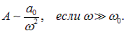
Physically this is understandable: the system possesses a certain inertia and does not have time to follow rapid changes of the external action. In the other limiting case of low external frequency

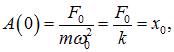
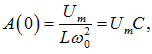
we are dealing with the static case — the action of a constant external force F0 on a spring pendulum, or the connection of the circuit to a source with constant voltage Um. In this case the limiting value of the amplitude of the forced oscillations equals

and does not depend on the damping. The latter is quite natural, since the damping is due to the action of the resistance force, which is proportional to the velocity and manifests itself only during motion of the system, not in the static limit. In the case of mechanical oscillations
|
|
|
(1.98) |
which equals the extension of the spring under the action of a constant force F0.
In the case of electromagnetic oscillations in the circuit
|
|
|
(1.99) |
which equals the charge on the capacitor when it is connected to a source of constant voltage Um.
Let us find the ratio of the resonant amplitude to the static amplitude for small damping, when  :
:
|
|
|
(1.100) |
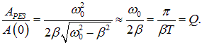
In other words, the quality factor Q also characterizes the resonant properties of the oscillatory system: the higher the quality factor, the higher and relatively narrower the resonance peak (see Fig. 1.26).
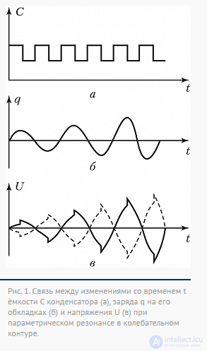
Self-oscillating systems. Parametric resonance.
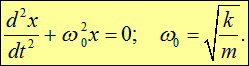
 .
.


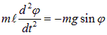






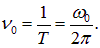
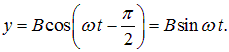
 — this is the number of oscillations performed by the system in unit time (in particular, in the SI system — per second).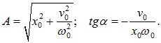













Comments