2.4. Standing waves - 2. Wave processes and elements of

Это продолжение увлекательной статьи про волновые процессы.

...

to kg/m³, we obtain the amplitude of the pressure oscillations at the pain threshold (L = 120 dB, I = 1 W/m²):

The amplitude of the displacement of the gas particles depends in this case on the frequency:

It follows from this that at a loudness of L = 120 dB and a frequency of n = 20 Hz the displacement amounts to A = 5.6·10^-4 m = 0.56 mm, while at a frequency of n = 20 kHz — A=5.6·10^-7 m = 0.56 µm.

Let us now find the amplitude of the velocity oscillation of the gas particles:

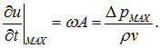
It does not depend on the frequency of the wave, and at a loudness of L = 120 dB it is equal to:

Table 1 presents the loudness levels for a number of sounds, with the help of which one can find the excess pressure, displacements, and velocities of gas particles in other cases.

Table 1

Loudness levels of some sounds

2.4. Standing waves

In addition to the traveling waves of the previous section, standing waves also exist in nature, formed as a result of the superposition of traveling waves. We constantly encounter them in our practical life: when we speak, sing, listen to music. In this section, after the general mathematical formulas, we will very briefly discuss some questions of musical acoustics – in the hope that this part will not seem to our students the most boring.

A string fixed at one end

Suppose that a string is fixed motionlessly at the point with coordinate and stretches in the positive direction of the x axis. Let a wave propagate along the string from right to left (that is, in the negative direction of the x axis)

Having reached the point of attachment, the wave will be reflected. If we neglect energy losses, the amplitude of the reflected wave coincides with the amplitude of the incident wave. It must also be taken into account that upon reflection the direction of motion of the element reverses (as in the elastic impact of a ball against a wall):

The superposition of the incident and reflected waves has the form:

We see that at any instant of time

This is precisely the condition for the string being fixed at the point . Using the well-known trigonometric formulas for the difference of cosines, we write (2.53) as:

where — the largest displacement in the standing wave.

We have found a special type of oscillation: at every point in space the string oscillates with frequency and amplitude , and all points of the string simultaneously reach their maximum deviations (or pass through the equilibrium position), and if we are, for example, at a node of the string, that is, at a point with coordinate

then at any instant of time this point remains a node. In other words, there is no motion of the wave here, the points of the wave's nodes (of zero displacement values) are stationary, as are the points of its maxima. Such oscillations are called standing waves.

This is obvious, if only because the points of the wave's nodes are stationary, and there can be no transfer of energy through them. One can also reason differently: the two traveling waves that formed the standing wave carry the same energy, but in opposite directions, so that these two processes mutually cancel each other.

Fig. 2.9 shows the formation of a standing wave when two monochromatic waves traveling toward each other are added together.

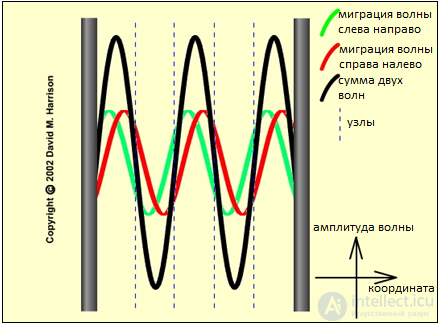
Fig. 2.9. Formation of a standing wave

Substituting the solution found (2.53) into expression (2.39), we obtain for the instantaneous value of the energy density of the standing wave the expression

Averaging over time, we find:

We have obtained that the average energy density of the standing wave does not depend on the point of observation and is equal to the sum of the average energy densities of the two traveling waves whose superposition it is.

Example 1. For a string fixed at one end, let us find the points at which the energy density of the oscillations does not depend on time.

Using the relation

we represent (2.54) as:

It is now clear that there will be no dependence on time if

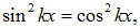
or

that is, at the points

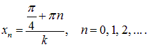
Example 2. Let us find the law of variation in time of the energy density of a standing wave at the points where the displacement of the string reaches its maximum values.

These points have coordinates

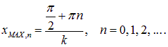
At these points

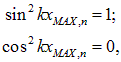
so that from (2.54) it follows:

Harmonics

On a string fixed at one end, oscillations of any frequency can exist. Let us now also fix the second end of the string at the point with coordinate . We have the same solution (2.53), which must satisfy the additional boundary condition:

This means that

On a string of length l, fixed at both ends, only standing waves with wave vectors can exist

Correspondingly, the wavelengths will be

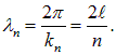
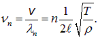
In other words, an integer number of half-wavelengths must fit along the length of the string. Consequently, a string fixed at both ends can oscillate only with certain frequencies:

Here we used equation (2.2) for the speed of waves on a stretched string.

From (2.58) it is seen that the oscillation frequency increases when:

• the length of the string decreases;
• its thickness (linear density) decreases;
• the tension increases.

These regularities are known to everyone who has ever held even a guitar. Oscillations with the lowest frequency (n = 1) are called the fundamental (first) harmonic, and those with subsequent frequencies are called the higher (second, third, etc.) harmonics.

Similar boundary conditions also exist for the oscillations of air in the pipes of wind musical instruments. Correspondingly, only quite definite frequencies are also present in their signals. Let us consider, for example, an organ pipe of length l. The pressure wave in it can also be described by an equation of the form (2.53):

If the pipe is open at both ends, then the pressure at the ends is equal to the stationary (atmospheric) pressure, and at the points x = 0, l. From this we obtain the same conditions for the wave numbers

the wavelengths

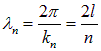
and the frequencies

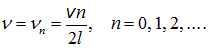
If, however, the pipe is open at the point x = 0 and closed at the other end (x = l), then at the closed end the displacement of the particles is equal to zero, while the pressure reaches a maximum or minimum:

From this somewhat different relations follow:

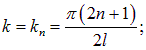
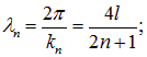
The first harmonic for such a pipe is excited at the frequency

which is two times smaller than the frequency

of the first harmonic of a fully open pipe.

Example 3. A nylon guitar string has a linear mass density of 7.2 g/m and is stretched with a force of 150 N. The length of the string is 90 cm. Let us determine what the four lowest frequencies obtainable on such a string are.

The wave velocity on the string is equal to

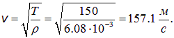
The greatest length of a standing wave in the string equals m. From this we find the lowest frequency:

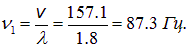
(This frequency corresponds to the note "F" of the great octave.)

The following frequencies are integer multiples of n₁:

Hence: n₁ = 2·87.3 = 174.6 Hz ("F" of the small octave), n₃ = 3·87.3 = 261.9 Hz ("C" of the first octave), and n₁ = 4·87.3 = 349.2 Hz ("F" of the first octave).

Example 4. A string sounds the note "C" of the first octave. The maximum displacement of the string's points from the equilibrium position equals u_max = 2 mm. Let us find the maximum velocity and acceleration of the string's points.

The law of vibration of the string has the form (cf. (2.53)):

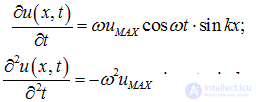
from which we find the velocity and acceleration of the string's points:

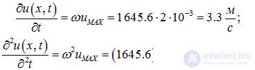
By the condition (see Example 3). The maximum values of the velocity and acceleration are equal to:

Addition of harmonics

Above we already dealt with the addition of vibrations, and now we must do the same, but for every point of the vibrating string.

The motion of the string when the fundamental (first) harmonic is excited is shown in Fig. 2.10–1. In the initial position (the line marked in red) the points of the string have the maximum displacement from the equilibrium position. Under the action of the elastic force they begin to move (vertically downward in the figure), and the shape of the string after 1/8 of a period is shown by the green line. After a quarter of a period the string arrives at the equilibrium position (the black line), but its elements have certain velocities, and therefore do not stay at the equilibrium position. After another 1/16 of a period they find themselves in the position shown by the blue line, and after half a period the string again acquires the maximum displacement (the dashed red line), but in the other direction, after which the process repeats in the reverse direction. This is how the vibration in the standing wave corresponding to the first harmonic occurs, whose frequency we denote n₁.

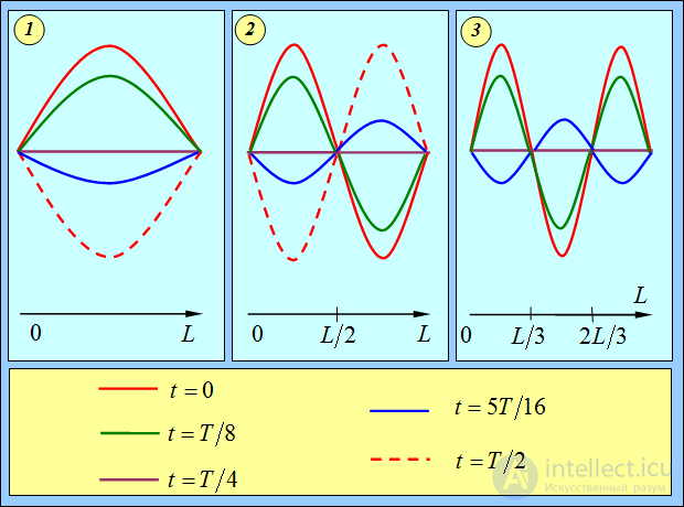
Fig. 2.10. Vibrations of the string:
1 – first harmonic; 2 – second harmonic; 3 – third harmonic;

But on the string, as we already know, vibrations of other harmonics can also arise. The second harmonic is shown in the same Fig. 2.10–2. Using the same notation lets us avoid describing the vibration process in as much detail. Note that in this case there is one fixed point (called a node) at the middle of the string. Since the node does not move anyway, we can imagine that we have fixed the middle point. And thereby, without changing the frequency of the emitted sound, we have shortened the string by half. Hence the vibration frequency is exactly twice the frequency of the fundamental harmonic: . We already obtained this result in another way.

Fig. 2.10–3 shows the vibrations of the same string when the third harmonic is excited. Here there are already two nodes, and the emitted sound corresponds to the fundamental vibration of a string shortened threefold (or, equivalently, to the second harmonic of a string whose length is 2/3 of the original): .

The vibrations of the string for the first three harmonics are shown in Fig. 2.11.

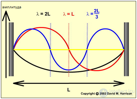
Fig. 2.11. Vibrations of the string for the first three harmonics

In the figures discussed, the harmonics are shown without regard to their amplitudes, that is, without regard to their relative contribution. In reality the contribution of the harmonics can vary, so that in the general case the resulting vibration is obtained by adding all the harmonics, each of which is represented by an equation similar to (2.59):

Here we have already taken into account that the frequencies and wave numbers take a discrete set of values; the coefficients – are the amplitudes of the corresponding harmonics. Note that in the time-dependent factor we replaced the sine with a cosine, that is, we shifted the origin of the time reference. Now at the moment t = 0 the velocities of all points of the string are zero.

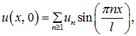
In practice one has to solve the inverse problem: to find the coefficients from the known resulting vibration. The numerical values depend on the way the string is excited, for example, on its initial shape . If we are given the function , then from (2.62) the expansion follows:

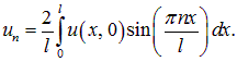
which is known in mathematics as a Fourier series expansion. It is also proved there that the coefficients u_n are uniquely recovered from the function :

The shape of the vibrating string depends on the amount of higher-harmonic admixture. Fig. 2.12 shows the shape of the vibrating string at different moments of time for two ways of exciting it. In both cases the string is given a certain initial shape, after which it is released "into freedom" (while remaining fixed at the ends, of course).

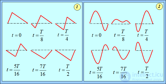
Fig. 2.12. Shape of the vibrating string at various moments of time for different shapes of the string in the initial state:
1 – the string is pulled aside a distance of 0.1 of its length; 2 – the string is given a piecewise-sinusoidal shape.

We consider two cases:

• in the initial position the string is pulled aside at a point located at a distance of 0.1 of its length, measured from its fixed end;
• the initial shape of the string is described by two sinusoids

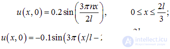
The second example is clearly of a model character and is given for comparison. It should be said that giving the string some initial shape is not the only way to excite vibrations. One can, for example, specify an initial velocity distribution (as happens, say, in a piano, where the hammer strikes the string that is at the equilibrium position).

Nevertheless we shall limit ourselves to the two cases described. Fig. 22.6 shows the positions of the points of the string over half a period of the fundamental harmonic's vibration, after which the process repeats in the reverse direction. In a time equal to the period of vibration T₁ of the first harmonic, the string returns to its initial position. If the string is tuned to the note "C" of the first octave, then T₁ = 3.82 ms.

Elements of music theory

1. Vibration spectrum. Timbre of sound, speech and singing

The intricate change in the shape of the string over time tells us little about the composition of the vibrations. Therefore perhaps the most important characteristic of a vibration is its spectrum: a diagram showing the relative contribution of each harmonic to the total intensity (energy) of the vibrations, that is, the function

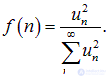
The spectrum of the vibration also depends on the way the string is excited. Fig. 2.13 gives a numerical calculation of the vibration spectrum of the string for both of our cases. The dark bars correspond to the "triangular" initial shape of the string, while the light bars show the vibration spectrum of a string whose initial shape is composed of pieces of different sinusoids. Along the horizontal axis the harmonic numbers are plotted, and the height of the bars along the vertical axis gives the relative intensity of the corresponding vibrations (that is, the share of each harmonic in the total intensity of the sound emitted by the string).

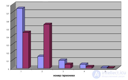
Fig. 2.13. Spectrum of the string's vibrations (first eight harmonics) for different ways of exciting the vibrations.
The blue bars show the amplitudes of the overtones for the "triangular" initial shape of the string,
and the purple bars — for the "piecewise-sinusoidal" shape

It can be seen that in the first case the greatest contribution comes from the first four harmonics — they account for 97.9 % of the sound intensity, the contribution of the next four harmonics is already small (2%), and all the rest account for only about 0.1% of the intensity. The specific numbers here depend on the way the string is excited; with a different method they may change. For example, when the string is pulled aside at the middle, all the even harmonics are simply absent from the spectrum; the first accounts for 98.55 %, the third — 1.22 %, the fifth — 0.16 %, and the remaining 0.07 % — for all the rest.

In the second case the contribution of the second harmonic is even greater than the contribution of the fundamental one, and the third and, to a lesser extent, the fourth harmonics are noticeable. In total, the contribution of the first four harmonics amounts to about 99.97 %, so that all the rest account for only 0.03 %.

These examples demonstrate a general rule: usually the lower harmonics of vibration are excited, while the influence of the higher ones decreases as their number grows. Depending on the presence of additional harmonics in the vibration spectrum (they are called overtones) the sound acquires its coloring, its timbre. The same note played on a flute, a violin, or an oboe is perceived differently. If a pure note were sounding, there would be no difference between one instrument and another. We owe the diversity of musical sounds to overtones. The degree of their presence, besides the way the vibrator is excited, also depends (and even to a much greater extent) on the resonator of the instrument. Thus, when playing the violin, the body of the instrument, vibrating under the action of the vibrations of the strings, and the volume of air inside the body take part in the formation of the sound. First, this amplifies the sound of the instrument: the main source of sound — the thin string — cannot by itself set in motion a large mass of air so that the sound reaches the listener. Second, vibrations arise on the top plate of the violin, and owing to resonance some overtones of the original string vibrations are amplified, while others — are damped. The resonators of musical instruments thus act as converters of the timbre of the original sound. It is well known that the value of an instrument, be it a violin or a grand piano, depends not on the quality of the strings stretched on it, but on the peculiarities of the structure of its body, of its plates. The art of the old Italian masters Stradivari, Amati, Guarneri, who made superb violins, violas and cellos, consisted, in particular, in the fact that they were able in practice to achieve an optimal vibration spectrum, which we perceive as the divine sound of their instruments.

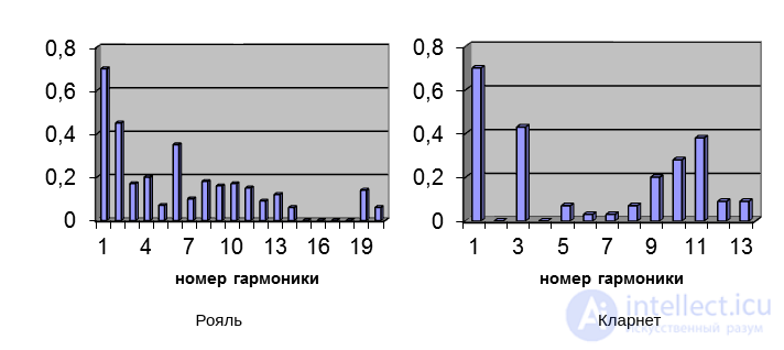
The regions where the higher overtones are amplified are called formants, and they determine the timbre of a given instrument. Fig. 2.14 shows the spectral decomposition of the sounds of a piano and a clarinet.

Fig. 2.14. Sound spectrum of various musical instruments

The formants are clearly visible in the spectrum: for instance, the sixth harmonic for the piano and the eighth–tenth for the clarinet. It is precisely these that create the differences in the sound of these instruments.

If we turn to the human voice, the source of the original sound is the glottis, the vibrations of the vocal cords (that is, in essence — the same strings). To the ear this sound differs sharply from the normal sound coming out of the mouth. It has a "squeaky" character and does not have the shape of any particular vowel sound, just as a simple guitar string does not have it: musical instruments cannot speak. The original timbre of the glottis acquires the character of speech sound as it passes through the oral-pharyngeal canal. Since the time of Helmholtz's acoustic research it has been known that every vowel sound contains in its spectrum two main, relatively amplified frequency regions — formants of vowels, or Helmholtz's characteristic tones. Our ear distinguishes one vowel sound from another by them. One of the frequencies is related to the resonance of the pharynx, the other — to the resonance of the oral cavity. The oral cavity is smaller in volume, and so the volume of air in it resonates at higher frequencies — of the order of kilohertz, while the pharyngeal cavity is larger in size, and it resonates at frequencies of the order of several hundred hertz. (The dependence of the resonant frequency on the size of the resonator cavity is the same as for the frequencies on a string — the shorter the string, the higher the frequency produced on it.) The change in the relative sizes of these cavities is produced by articulation of the tongue, whose movement creates in the oral and pharyngeal cavities the air volumes needed for the formation of formants. In old times criminals had their tongues cut out, and they lost the ability to pronounce vowel sounds, lost the gift of speech, although their voice was preserved. The formants for the vowels of the Russian language have approximately the following values: i – 240 Hz and 2,250 Hz, u – 300 Hz and 650 Hz, e – 440 Hz and 1,800 Hz, o – 535 Hz and 780 Hz, a – 700 Hz and 1,000 Hz. In women and children the formant regions are shifted somewhat toward higher frequencies, and thanks to this we distinguish who is speaking to us, even if the frequency of the fundamental tone is the same. It is important that the formant regions remain constant despite a change in the pitch of the fundamental tone: a person can pronounce the vowel e in a bass or a light tenor voice, but the formant frequencies will be the same (Fig. 2.15). Some discrepancies in the numbers between the data given and the figure are due to the fact that the measurements differ slightly among different groups of researchers.

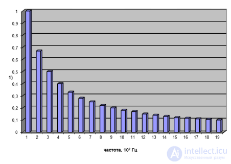
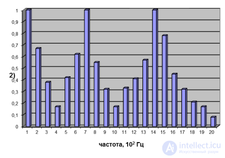
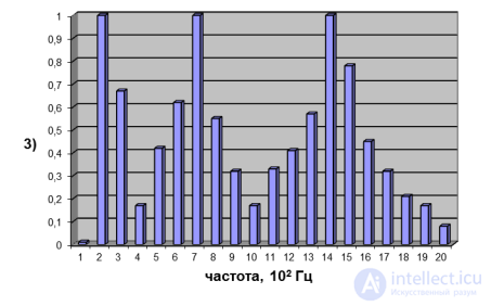
Fig. 2.15. Spectrum of the larynx, consisting of overtones that decrease uniformly in amplitude (1), and spectra of the sound e,
taken at a frequency of 100 Hz (2) and 200 Hz (3). The formant regions n = 700 Hz and n = 1,400 Hz
remain unchanged despite the change in the pitch of the fundamental tone

In the study not of speech, but already of singing, two more regions of overtones were discovered — the so-called singer's formants. In the 1920s–1930s it was found that in the spectrum of a well-trained male voice there are always amplified overtones with a frequency in the region of 500 Hz. The presence of this low singer's formant gives the voice a rounded, full and soft sound. The high singer's formant lies in the region of 3,000 Hz; it brings brightness, brilliance to the sound, creates a silvery timbre. In masters of the vocal art, up to 30–35 % of the entire sound energy of the voice is concentrated in the region of the high singer's formant, whereas in speech, even trained speech (of announcers and actors) — only 5–7 %. The more intense the sound, the more pronounced the singer's formants become compared to the formants of vowels. Therefore at high sound power the vowels become poorly distinguishable, and we recognize them more by context, at the initial moment of the sound's formation. Fig. 2.16 shows the spectrum of the voice of F. Chaliapin.

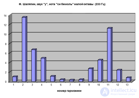
Fig. 2.16. Spectrum of the voice of F. Chaliapin. The fundamental tone plays essentially no role in Chaliapin's overall spectrum.
Its amplitude is taken in the figure as unity. The main energy is concentrated in the low singer's formant — 2–4 overtones.

The high singer's formant arises in the human larynx — in the supraglottic cavity between the vocal cords and the entrance to the larynx. This cavity has dimensions of the order of 3 cm, which at a speed of sound of v = 340 m/s leads to resonance at a frequency of

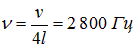
(the fundamental tone of a closed pipe, which we discussed above), that is, precisely in the region of the high singer's formant. The place of origin of the low singer's formant has not been precisely determined: the data point most likely to resonance of the tracheal tube.

The quality of "carrying power" is associated with the timbre of the voice, with the presence in its spectrum of high overtones. There exist singing voices that fly across the hall and "pierce through" the sound of the orchestra, and sometimes they do not have great power. And conversely, there are voices of extraordinary power that get lost in large rooms, drowned out by the sound of the orchestra. The quality of carrying power turned out to be related to the peculiarities of our hearing, which is most sensitive to the frequency region of 2,500 – 3,000 Hz. The outer auditory canal of the ear resonates at these frequencies, and such sounds are subjectively perceived as louder. As we already know, this is the region of the high singer's formant. Voices in which a large percentage of the energy is concentrated in the high singer's formant have the ability to "fly through the orchestra"; they are well heard in a large hall.

2. Pitch of sound and the structure of the musical scale

Equal temperament

One of the most important characteristics of a musical sound is its pitch, whose quantitative measure is the frequency n of vibration of the corresponding vibrator (a column of air in wind instruments, a string — in string instruments, and so on). The frequency of vibration can take any values, but from the standpoint of the perception of a musical sound a certain periodicity is observed: two sounds are perceived as similar if the frequency of one of them is exactly twice the frequency of the other. This axiom of equivalence of sounds was proclaimed in 1722 by the French composer Jean-Philippe Rameau. Such two sounds correspond to the same note, and, as it is said, they are separated by an interval called an octave.

The international standard for the note "A" of the first octave sets the frequency Hz. The note "A" of the next, second, octave has a frequency exactly twice as large — Hz. In the European system the octave is divided into twelve different sounds (recall, for example, the seven white and five black keys in each octave of the piano). The interval between neighboring sounds is called a semitone. How, then, should the corresponding vibrators be tuned, starting from the standard frequency ? One way — equal temperament (as musicians say – equal temperament), in which the ratio between the frequencies of neighboring sounds is constant. This ratio, as is easy to see, equals

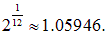
It is precisely this number, when multiplied by itself 12 times, results in a doubling of the frequency for the same note in the next octave:

Having adopted the equal-tempered system, we can calculate the frequencies of any notes. Thus, the note "A" of the first octave and the note "C" of the second octave are separated by three semitones, that is, the frequency of the latter must equal

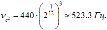
Accordingly, the frequency Hz of the note "C" of the first octave is obtained from this by dividing by two. The note "G" of the first octave is seven semitones away from "C" of the same octave, that is, its frequency equals

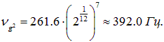
The results of similar calculations for four octaves are given in Table 2.2.

Table 2.2.

Pitch of musical sounds in the equal-tempered system: for each note its international (Latin) designation and frequency in hertz are given

Let us note, incidentally, that these octaves were chosen for the example not by chance: it is precisely in this range that the human voice lies. The highest female singing voice — soprano — is characterized by the range c¹–e³ (rarely — up to g³). A few tones lower lies the range of mezzo-soprano: a–h². The lowest female voice — contralto — has a typical range of f–a². Countertenors deserve special mention — present-day performers of works once written for castrato singers. But the range of the latter was extraordinarily wide, and few of today's singers can fully reproduce the once-popular works. "Typical" countertenors (if one can speak of typicality for such rare voices) sing in the range (c–e²), differing from contralto in timbre.

The highest of the ordinary male voices — tenor — typically has the range c–c². Next come baritone (A–f¹) and bass (C–e¹). Thus "vocal" frequencies extend from about 70 Hz to 1,400 Hz (here we are talking about the fundamental note, not the admixture of overtones). Approximate ranges of singing voices are shown in Fig. 2.17 together with the ranges of string instruments — violin, viola, cello and double bass. The king of instruments — the concert grand piano — usually spans 7.25 octaves: from A₂ (27.5 Hz) to c⁵ (4,186 Hz).

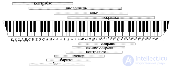
Fig. 2.17. Approximate ranges of string instruments and human voices

The idea of equal temperament was born in Germany at the turn of the 17th–18th centuries. The proposed musical scale initially met with resistance, but after J.S. Bach composed, in 1722–1744, "The Well-Tempered Clavier" — a collection of preludes and fugues, one for each of the existing 24 keys — the viability of the new scale was proven. Since then it has become universally accepted. The main advantage of the equal-tempered scale is the possibility of transposing a melody into another range without distorting it. For example, the melody "Chizhik" (e¹ – c¹ – e¹ – c¹ – f¹ – e¹ – d¹), played in the first octave, corresponds to the sequence of frequencies (in Hz): 330–262–330–262–349–330–294 (we have rounded the values given in Table 3.2). Suppose we want to play it, shifting the start up by three keys — from the note "B", which corresponds to a frequency of 494 Hz. The ratio of the first notes of the original and transposed melodies equals 493.7/329.6=1.4983=2^7/12 (the exponent corresponds to the seven semitones separating the notes "E" and "B" — see Fig. 3.17). The ratio of the second and all subsequent notes of the melody must be the same. Hence the sequence of frequencies of the transposed melody must have the form 494–392–494–392–523–494–440, that is, the transposed melody will sound as b¹ – g¹ – b¹ – g¹ – c² – b¹ – a¹.

Why, then, did the equal-tempered musical scale meet with objections? The fact is that already in antiquity, since the time of Pythagoras, it was known that certain notes, taken simultaneously, sound in consonance, harmoniously, not conflicting with one another. Pythagoras counted among such two-note combinations the octave (frequency ratio 2:1), the fifth (3:2) and the fourth (4:3) — the so-called perfect consonances. Later the major and minor thirds (5:4 and 6:5) were also added to them. What, then, is common between the consonance of a two-note combination and the ratio of the first six integers?

Let us work out what happens when two notes are taken simultaneously. The lower-pitched sound is called the root of the interval, the upper one — its top note. Let the root correspond to a frequency v₁ when the string sounds this note, the first overtones with frequencies v₂ = 2v₁, v₃ = 3v₁, v₄ = 4v₁ will inevitably also be excited. If now, simultaneously with the first note, we take another one, forming an octave interval with the first (its corresponding frequency being v₂ = 2v₁), then overtones with frequencies v₄=2v₂ = 4v₁, v₆ = 3v₂ = 6v₁, and so on, will also arise on it. We see that the composition of the sonority has, in essence, not changed — the addition of the new note has not added any new overtones. That is why the octave sounds almost like a single note, an absolute consonance.

An "admixture" of the second harmonic always exists in the vibration of any vibrator, and perhaps this is the reason why our ear perceives identical notes in different octaves as sounding in unison, as, in essence, the same note. Herein, apparently, lies the physical basis of Rameau's axiom of equivalence, the very concept of the octave as a certain measure of the periodicity of a musical sound, when the same notes begin to repeat.

In passing we established that the note corresponding to the frequency v₃ = 3v₁ is closely related to the note originally taken — one way or another, this sound is already present in the original as its third harmonic. But by the equivalence theorem, the frequency

продолжение следует...

Продолжение:

Часть 1 2. Wave processes and elements of music theory
Часть 2 2.4. Standing waves - 2. Wave processes and elements of
Часть 3 2.5. Spherical waves - 2. Wave processes and elements of
Часть 4 - 2. Wave processes and elements of music theory