
Lecture
Это продолжение увлекательной статьи про волновые процессы.
...
v1quint=3v1/2 corresponds to this note in the preceding octave. Thus the interval in which the root corresponds to the frequency v1, and the top note — to the frequency vquint = 3n1/2, will be consonant. Such an interval is called, as we recall, a fifth, and the ratio of the frequencies of the top note and the root in a fifth is exactly equal to 3/2.Let us now take the consonant fifth — a two-note combination with frequencies v1 and vquint = 3v1/2, — and add to it a third note forming an octave with the root. Its frequency equals 2v1. By the equivalence theorem, the consonance of this sonority will not be disturbed. But if the interval between the root and the third note (an octave) is consonant, and the interval between the root and the top note of the two-note combination (a fifth) is consonant, then the interval between the top note and the third note must also be consonant. The corresponding frequency ratio equals v2/vquint = 2v1/(3v1/2) = 4:3. Such an interval is called, as we recall, a fourth. If we take as the root of the interval the same note with frequency v1, then the note forming a fourth with it sounds at the frequency vquart = 4v1/3.
In principle, these ratios of integers could be taken as the basis for constructing a musical scale. But then a problem would arise with transposing a melody.
Let us try to construct one octave of a hypothetical musical scale, a) based on the ratio of whole numbers, and b) allowing the melody to be transposed. Suppose this scale contains some note with frequency v. Then it must also contain a note forming an octave interval with the original (2v). Suppose also that the scale contains another note forming, say, a perfect fifth with the first (3v/2). Then the scale must also contain a note two fifths away from the first: its frequency equals (3/2)2v = 9v/4, and lowering it by an octave gives us the note 9v/8. Lowering a combination of three fifths by an octave leads to a note with frequency v/(3/2)3/2 = 27v/16, and lowering a combination of four fifths by two octaves leads to the frequency 81v/64, and so on. Continuing this process, we obtain an infinite number of notes within a single octave, because no power of three can ever equal a power of two (an odd number cannot equal an even number). Hence the described procedure keeps producing new and new notes that must be included in the scale. The same result is obtained if the scale is built on fourths rather than fifths. Thus requirements a) and b) for a musical scale turn out to be incompatible. One of them must be dropped, and it is simpler to sacrifice the whole-number ratio for perfect consonances, gaining freedom to choose keys and ease of transposing melodies.
For this reason musicians abandoned tuning their instruments according to the law of whole-number ratios, and switched to equal temperament. In this case the frequencies of perfect consonances are reproduced only approximately. For example, in an equally tempered scale the fifth corresponds to an interval of 7 semitones: 27/12 = 1.4983, which differs from the pure fifth (a ratio of 1.5) by only 0.1 %. Such is the interval, for example, between the notes "C" and "G." The fourth corresponds to an interval of 5 semitones: 25/12 = 1.3348, which also differs from the pure fourth (1.3333) by 0.1 % (a trained ear can hear even such small deviations from the ideal intervals).
It would be interesting to discuss the physical principles underlying the major (C–E–G) and minor (C–E flat–G) triads, but this would take us too far from physics, to which it is time to return. We hope, however, that these musical examples have helped in mastering the important concepts of higher harmonics and the vibration spectrum, which we shall meet again.
In the previous sections we considered a special type of wave: the phase
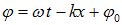
depended only on the coordinate x.
|
Wave front — is a non-stationary surface, at every point of which the wave phase has the same value, constant in time. |
For the waves we have studied, the oscillations of the medium are the same at all points of the plane orthogonal to the direction of wave propagation (which we chose as the x axis). In other words, the wave front is a plane parallel to the plane containing the y, z axes. The front of a traveling wave moves over time along the x axis with phase velocity v. Such waves are called plane waves.
Three-dimensional wave equation
Let us still deal with a plane wave. Let us rotate the coordinate axes so that the direction of wave propagation is given by some unit vector n. The solution obviously has the form:
|
|
|
(2.65) |
The relations between  , k and
  remain the same.
|
Wave vector — is a vector whose magnitude equals the wave number, and whose direction coincides with the direction of wave propagation:
|
The wave front – a plane orthogonal to the wave vector k, – moves with velocity v, remaining parallel to itself.
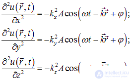
Let us find the equation satisfied by solution (2.65). We differentiate expression (2.65) twice with respect to the coordinates x, y, z:
|
|
|
(2.66) |
Adding these three equations, we find:
|
|
|
(2.67) |
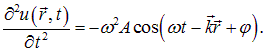
The second time derivative of the solution has the form:
|
|
|
(2.68) |
Taking into account the relation

we obtain from (2.67), (2.68):
|
|
|
(2.69) |
The expression in brackets on the left-hand side of the equation is a differential operator called the Laplacian (or Laplace operator) and has the special notation  .
.
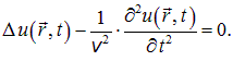
We write the wave equation for waves in three-dimensional space in its final form:
|
|
|
(2.70) |
If the wave function u depends only on one coordinate (say, x), then the Laplacian turns into the second derivative with respect to x, and we return to the previous form of the wave equation.
Let us emphasize that is not the Greek letter ("delta"), and u is not the increment of the quantity u, but the sum of its second derivatives with respect to the coordinates.
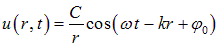
But the wave equation (2.70) has other solutions besides plane waves. By simple differentiation one can verify that the spherical wave
|
|
|
(2.71) |
satisfies the wave equation. The wave front is a sphere centered at the location of the source of oscillations (r = 0), the radius of the sphere increasing with velocity v.
Indeed, the surface of constant phase is given by the equation

differentiating which, we find

The amplitude of the spherical wave

decreases with increasing distance to the observation point. The intensity of the wave

decreases according to the inverse-square law. This, like Coulomb's law, is also related to the three-dimensionality of our space. If the medium does not absorb the radiation, then the energy flux through the surface of a sphere is the same for spheres of any radius surrounding the radiation source. Since the area of the sphere equals 4pr2, the energy passing through a unit area is inversely proportional to r2.
Standing by the railway track, one can observe the following phenomenon: the signal of an approaching train sharply changes its pitch (frequency) at the moment the train passes the observer. The same phenomenon can be noticed by an observer sitting in a train and passing a honking car standing at a crossing.
Fig. 2.18 demonstrates a similar phenomenon when a helicopter moves past an observer.
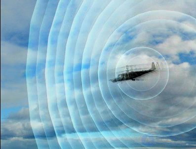
Fig. 2.18. Change of sound pitch as a helicopter moves past an observer
|
Doppler effect — is the change in the observed frequency of a wave due to relative motion of the source and/or the observer. |
The effect is named after the Austrian physicist C. Doppler, who predicted it theoretically in 1842.
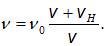
Moving observer, stationary sound source. Suppose there is a sound source emitting spherical sound waves. Fig. 2.19 shows the arrangement in space of four consecutive crests (maxima) of the sound waves. Let the wave have frequency  , then the distance between crests equals the wavelength

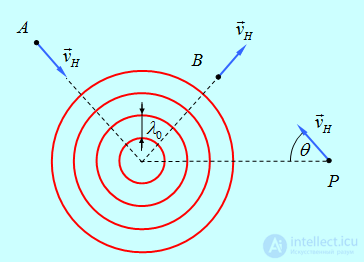
Fig. 2.19. Doppler effect for a moving observer
Observer A moves straight toward the sound source with velocity  . Therefore the wave crests approach him with an increased speed
  . The observer will meet each successive wave crest after a time

after the previous one. Hence the period of oscillation changes for him. The observed wave frequency equals
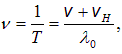
from which we find:
|
|
|
(2.72) |
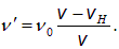
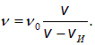
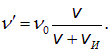
Observer B moves away in a straight line from the source with the same speed  (we assume that
  , an observer moving away from the source at supersonic speed would "outrun" the wave and would not hear the sound at all). So the wave crests approach him with speed
  , and the period of oscillation equals

From this we obtain for the observed frequency:
|
|
|
(2.73) |
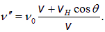
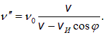
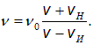
Finally, let observer P move with velocity vH, making an angle  with the direction toward the source. Only the velocity component along the line joining the observer and the source affects the frequency shift:
|
|
|
(2.74) |
The previous formulas (2.72) and (2.73) are obtained from this for the special cases at  and
and  , respectively.
Fig. 2.20 uses a model to demonstrate the Doppler effect for the case of a stationary sound source and a moving observer.
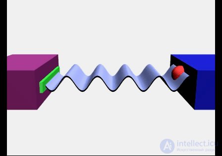
Fig. 2.20. Modeling the Doppler effect for a moving observer
Moving sound source, stationary observer. Suppose now that the observer is stationary, and sound waves are emitted by a source moving with velocity  . Fig. 3.21 shows the arrangement in space of four consecutive crests of the sound wave, marked with the black numbers 1, 2, 3, 4.
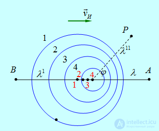
Fig. 2.21. Doppler effect for a moving source
These crests were emitted when the sound source was at the points marked with the red numbers 1, 2, 3, 4, respectively. In other words, point 1 is the center of sphere 1, point 2 — the center of sphere 2, and so on. It can be seen that the centers of neighboring spheres are shifted by the distance traveled by the source during a period of oscillation

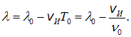
This leads to a change in the distance between the wave crests arriving at the observer. Consequently the observer registers a different wavelength.
Observer A is positioned so that the source moves directly toward him. For this observer the distance between wave crests decreases and equals
|
|
|
(2.75) |
The wave speed does not depend on the motion of the source, since it is determined by the properties of the medium. Hence we have the usual relation between the wavelength and its phase velocity:
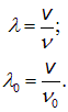
Substituting these relations into (2.75), we obtain

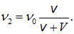
from which we find the frequency n of the sound perceived by observer A:
|
|
|
(2.76) |
For observer B the distance between wave crests increases and equals
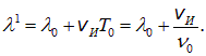
Similar reasoning leads to the following expression for the frequency of the sound wave:
|
|
|
(2.77) |
Finally, for observer P, for whom the direction makes an angle  with the velocity of the source, the expression for the frequency has the form:
|
|
|
(2.78) |
The previous expressions are obtained from this at  and
and  , respectively.
Example 1. An observer standing on a railway platform hears the horn of a passing train. When the train is approaching, the frequency of the horn's sound vibrations equals  , and when the train is moving away —
  . Let us determine the speed of the train V and the horn's own frequency
  . The speed of sound v is assumed to be known.
With train speed V, sound speed v and natural oscillation frequency  , the frequency
  , perceived as the train approaches, equals
|
|
|
(2.79) |
As the train moves away, the perceived sound frequency equals
|
|
|
(2.80) |
Dividing the first relation by the second, we obtain:
|
|
|
(2.81) |
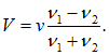
From this we find the speed of the train:
|
|
|
(2.82) |
Substituting the train's speed into expression (2.79), we obtain from it:
|
|
|
(2.83) |
Fig. 2.22 uses a model to demonstrate the Doppler effect for a moving sound source and a stationary observer.
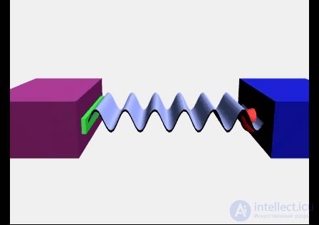
Fig. 2.22. Modeling the Doppler effect for a moving source
Moving sound source, moving observer. From the formulas obtained we can draw general conclusions:

|
|
|
(2.84) |
 and
and  should now be understood not as the absolute velocities of the observer and source, but as their projections onto the line joining the source and observer: positive signs of the velocities correspond to approach, negative — to the source and observer moving apart.
Expression (2.84) explicitly violates Galileo's principle of relativity. Indeed, the speed  of approach of the source and observer is the sum of the corresponding velocity projections:
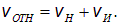
According to the principle of relativity, all observed effects should depend only on  . Formula (2.84), however, allows us to separate the motion of the observer from the motion of the source. To illustrate this, let us consider three examples. We hasten to reassure the reader: this is an apparent puzzle, and its explanation is given below at the end of the discussion of example 4. Galileo's principle is perfectly fine.
Example 2. The siren of a police car standing on the shoulder of the road emits a signal at a frequency of 1,000 Hz. Let us determine what frequency of sound will be heard by a driver passing by at a speed of 80 km/h.
In this case the speed of the car V = 80 km/h = 22.2 m/s — is the speed of the observer. The speed of sound is  . As he approaches the police car, the driver perceives a sound of frequency

After the driver has passed the police car, the perceived frequency becomes equal to

Example 3. The driver of a car standing on the shoulder of the road notices a police car passing by with its siren on. Let us find the frequency of the sound heard by the driver, if the speed of the police car is 80 km/h. The police siren is the same as in the previous example.
Here the speed V = 22.2 m/s — is the speed of motion of the source. As the police car approaches, the driver hears a signal of frequency

As it moves away, the frequency of the perceived signal equals

Example 4. The same two cars are driving toward each other with equal speeds of 40 km/h = 11.1 m/s. Let us find the frequencies of the sound signal as the cars approach and as they move apart.
We apply formula (2.84). As they approach, the perceived sound has frequency

As the cars move apart, the siren sounds to the driver at frequency

In all three cases we obtained different results, although each time the speeds of approach (recession) of the observer and the source were the same. At the same time, the numerical results are close to one another. This is explained by the fact that the speeds of the cars in the problem are small compared with the speed of sound. In this case, in formula (2.84) we can neglect terms

and higher powers. Let us transform (2.84):
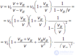
Now neglecting the terms containing ratios of squared velocities, we find the approximate expression:
|
|
|
(2.85) |
In (2.85) the frequency depends only on the relative velocity of the source and observer. If the formula were exact, in all three problems we would have obtained the same answer:
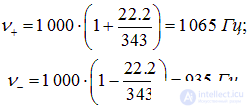
Formula (2.85) satisfies Galileo's principle of relativity, but, strictly speaking, it is exact only for an infinitely large signal speed. The violation of Galileo's principle of relativity is related to the presence of a medium. Indeed, when bodies move through a medium, one can distinguish a state of rest from uniform straight-line motion at least by the wind that arises due to the motion. Therefore, in the presence of a medium, reference frames are not equivalent: among them, the one in which the medium as a whole is at rest is singled out.
Let us now consider the case in which the source of sound waves moves with a speed exceeding the speed of sound:  . Let at time t = 0 the source be at point S0, and at time t it is at point St (Fig. 2.23). The distance between these points equals
  .
.
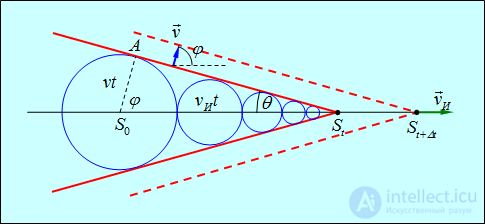
Fig. 2.23. Formation of the Mach cone for supersonic motion of the source
At every point of its trajectory (for simplicity we consider uniform straight-line motion), the source emitted spherical sound waves. The wave emitted at time t = 0 has, by the current time t, reached point A. The waves emitted along the path from S0 to St have managed to travel shorter distances. As can be seen from Fig. 2.23, at a given moment in time there is a conical surface (called the Mach cone), tangent to the fronts of all the emitted spherical waves. This conical surface starts at the sound source, and its axis coincides with the direction of motion of the source. The Mach cone separates the regions of space that the sound from the source has reached from those regions that the sound has not yet reached. At the next moment of time  the source will move to point
  . Accordingly, the Mach cone will also move, capturing new regions of space (shown by the dashed line).
The sine of the cone's half-angle is defined as the ratio of the distance  , traveled by the sound wave in time t, to the distance
  , traveled by the source in the same time:
|
|
|
(2.86) |
The conical surface can be regarded as a wave front (it is called the shock front). The direction of wave propagation is the normal to the front. Consequently, the shock wave propagates at an angle

to the direction of motion of the source. Accordingly, (2.86) can be written as:
|
|
|
(2.87) |
|
Mach number — is the ratio |
Example 5. An airplane flies horizontally at an altitude of 5,000 m at constant speed. An observer noticed it directly overhead, and recorded the time. The sound from the airplane appeared 11 s after that. Let us find the speed of the airplane and determine at what horizontal distance the airplane is from the observer at the moment the latter registers the arrival of the sound from it.
During time t the airplane moved away from the observer by a distance  . Since at this moment the sound reached the observer, the observation point turned out to be on the Mach cone (Fig. 2.24).
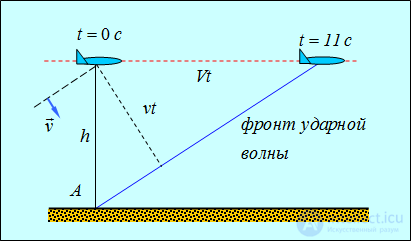
Fig. 2.24. On example 5. Concerning the flight of a supersonic airplane. The dashed line – position of the Mach cone
at the moment the airplane flies overhead, the solid line – the Mach cone at the moment
when the sound reaches the observer
We have the relations:
|
|
|
(2.88) |
From this:
|
|
|
(2.89) |
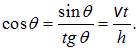
Using the relation
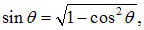
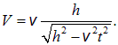
we obtain the relation between the airplane's speed, its flight altitude, and time t:
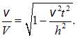
from which:
|
|
|
(3.90) |
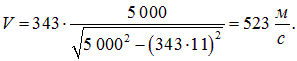
Substituting the numerical data:
|
|
|
(3.91) |
The Mach number (here  ) equals
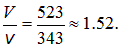
At this speed of motion, the airplane has moved away horizontally by a distance

Let us note, incidentally, that the moment the shock wave front reaches the observer is perceived as a sharp bang (similar to thunder). The common expression "the airplane broke the sound barrier" does not correctly reflect the physical process: the bang, as we have seen, is not related to the moment the airplane acquired supersonic speed.
Fig. 2.25 demonstrates the passage of a shock wave as a supersonic airplane moves.
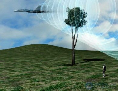
Fig. 2.25. Passage of a shock wave during the motion of a supersonic airplane
Let us analyze formula (2.90). It can be seen that the delay time t cannot be greater than

Such a delay could occur at a very high speed of the airplane (V>>v), when the Mach cone becomes extremely narrow, almost parallel to the direction of motion. The shock wave front, propagating vertically downward, must in this case travel a distance h, which it does in time  .
.
A delay time of t = 0 corresponds to the case in which the airplane's speed equals the speed of sound: V = v. In this case the half-angle of the Mach cone becomes equal to  (Fig. 2.26), so that the shock wave reaches the observer at the very moment the airplane is directly overhead.
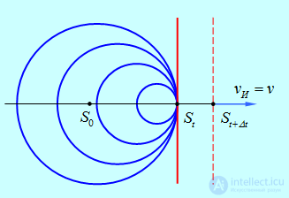
Fig. 2.26. Shock wave front in the case of a source moving at the speed of sound. At every moment of time t the source lies on the surface of all the spherical waves emitted earlier. The envelope of these spherical waves – the shock wave front – is a plane orthogonal to the direction of motion of the source
At subsonic speeds the sound outruns the aircraft and reaches the observer before the airplane does.
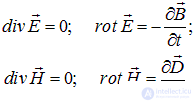
Any oscillatory circuit radiates energy. A changing electric field excites a variable magnetic field in the surrounding space, and vice versa. The mathematical equations describing the relation between the magnetic and electric fields were derived by Maxwell and bear his name. Let us write Maxwell's equations in differential form for the case when there are no electric charges ( ) and currents (j = 0):
|
|
|
(2.92) |
where

The quantities  and
and  — are the electric and magnetic constants, respectively, which are related to the speed of light in vacuum by

The constants  and
and  characterize the electric and magnetic properties of the medium, which we shall assume to be homogeneous and isotropic.
In the absence of charges and currents, static electric and magnetic fields cannot exist. However a variable electric field excites a magnetic field, and conversely, a variable magnetic field creates an electric field. Therefore there exist solutions of Maxwell's equations in vacuum, in the absence of charges and currents, in which the electric and magnetic fields turn out to be inseparably linked to one another. In Maxwell's theory, two fundamental interactions previously considered independent were united for the first time. That is why we now speak of the electromagnetic field.
An oscillatory process in a circuit is accompanied by a change in the field surrounding it. The changes occurring in the surrounding space propagate from point to point with a certain speed, that is, the oscillatory circuit radiates electromagnetic field energy into the surrounding space.
|
Electromagnetic wave — is an electromagnetic field propagating in space, in which the electric field strength and the magnetic flux density change according to a periodic law. |
When the vectors  and
and  vary strictly harmonically in time, the electromagnetic wave is called monochromatic.
Let us obtain wave equations for the vectors and from Maxwell's equations.
Wave equation for electromagnetic waves
As already noted in the previous part of the course, the curl (rot) and divergence (div) — are certain differentiation operations, performed according to definite rules on vectors. Below we shall become better acquainted with them.
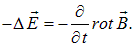
Let us take the curl of both sides of the equation
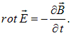
Here we shall use the formula, proved in the mathematics course:

where  — is the Laplacian introduced above. The first term on the right-hand side is zero by virtue of another of Maxwell's equations:

As a result we obtain:
|
|
|
(2.93) |
Let us express rotB in terms of the electric field using Maxwell's equation:
|
|
|
(2.94) |
and use this expression on the right-hand side of (2.93). As a result we arrive at the equation:
|
|
|
(2.95) |
Taking into account the relation

and introducing the refractive index of the medium

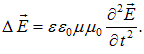
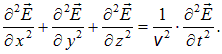
we write the equation for the electric field strength vector in the form:
|
|
|
(2.96) |
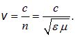
Comparing this with (2.69), we see that we have obtained the wave equation, where v — is the phase velocity of light in the medium:
|
|
|
(2.97) |
Taking the curl of both sides of Maxwell's equation

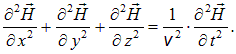
and proceeding in a similar manner, we arrive at the wave equation for the magnetic field:
|
|
|
(2.98) |
The wave equations obtained for  and
and  mean that the electromagnetic field can exist in the form of electromagnetic waves, whose phase velocity equals
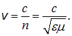
In the absence of a medium (at  ) the speed of electromagnetic waves coincides with the speed of light in vacuum.
Main properties of electromagnetic waves
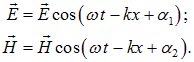
Let us consider a plane monochromatic electromagnetic wave propagating along the x axis:
|
|
|
(2.99) |
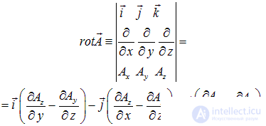
The possibility of the existence of such solutions follows from the wave equations obtained. However, the strengths of the electric and magnetic fields are not independent of one another. The relation between them can be established by substituting solutions (2.99) into Maxwell's equations. The differential operation rot, applied to some vector field A, can be written symbolically as a determinant:
|
|
|
(2.100) |
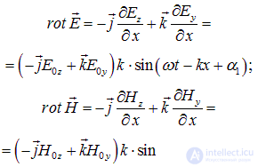
Substituting expressions (2.99) here, which depend only on the coordinate x, we find:
|
|
|
(2.101) |
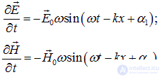
Differentiating plane waves with respect to time gives:
|
|
|
(2.102) |
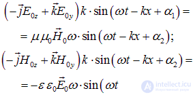
Then from Maxwell's equations it follows that:
|
|
|
(2.103) |
From this it follows, first, that the electric and magnetic fields oscillate in phase:

Further, neither  , nor
, nor  has components parallel to the x axis:
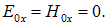
In other words, also in an isotropic medium,
|
electromagnetic waves are transverse: the oscillations of the electric and magnetic field vectors occur in a plane orthogonal to the direction of wave propagation. |
Then we can choose the coordinate axes so that the vector  is directed along the y axis (Fig. 2.27):

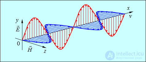
Fig. 2.27. Oscillations of the electric and magnetic fields in a plane electromagnetic wave
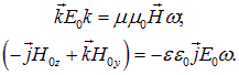
In this case, equations (2.103) take the form:
|
|
|
(2.104) |
It follows that the vector  is directed along the axis z:

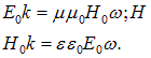
In other words, the electric and magnetic field vectors are orthogonal to each other and both — to the direction of wave propagation. Taking this fact into account, equations (2.104) simplify even further:
|
|
|
продолжение следует...
Часть 1 2. Wave processes and elements of music theory
Часть 2 2.4. Standing waves - 2. Wave processes and elements of
Часть 3 2.5. Spherical waves - 2. Wave processes and elements of
Часть 4 - 2. Wave processes and elements of music theory

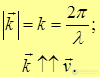


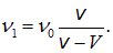





 , that is the speed of the source to the speed of sound in the given medium.


Comments