
Lecture
Это продолжение увлекательной статьи про уравнение шредингера.
...
quantum numbers  1, 2 and 3, which, as before, take integer values. Here we encounter for the first time the important concept of degeneracy of energy levels, that is, a situation in which different states of the system have the same energy. Indeed, the minimum energy of the system is reached at the minimum values of all the quantum numbers, that is, at 1, 2, 3. This energy equals

and it corresponds to a single wave function  . It is said that the ground state is non-degenerate (non-degeneracy of the state with minimum energy is a general rule). The first excited state is obtained when one of the quantum numbers equals 2, while the others remain equal to unity; its energy is

But now three states with wave functions  ,
,  , and
, and  have this energy (the quantum number 2 can be chosen in three ways), so it is said that the degree of degeneracy of the first excited level equals three (g = 3). Naturally, another system may have an entirely different degree of degeneracy (or none at all). The subsequent states of a particle in a three-dimensional potential well with infinite walls are likewise degenerate. It is clear that the degeneracy of levels is connected with the symmetry of the system, with the equivalence of all axes. If the dimensions of the well were different
  1, 2, 3 along the three directions, then instead of (4.27) we would obtain for the energy the expression
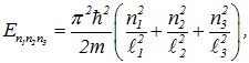
and degeneracy could occur only for certain ratios between the length, width, and height of the potential box.
One-dimensional oscillator
In classical physics a spring pendulum (one-dimensional oscillator) is a point body of mass m, attached to a spring and oscillating with angular frequency  . The potential energy of such a system is described by the expression
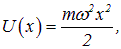
so that the Schrödinger equation is written as

From this we can find the solution for the ground-state wave function
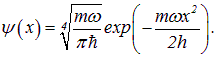
Substituting this expression into the Schrödinger equation, it is easy to verify that the ground-state energy equals

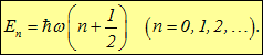
We shall not write out the wave functions of the excited states of the oscillator, but the expression for the allowed energy values has the form ( is the vibrational quantum number)
|
|
|
(4.28) |
Here Planck's formula is reproduced, together with zero-point oscillations
 ,
,
obtained earlier from the uncertainty relations (see Sec. 3.3).
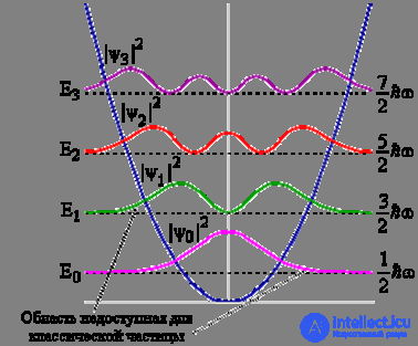
Fig. 4.10. Energy levels and probability density distributions over the coordinate x for different values of the vibrational quantum number. The potential-energy curve of the oscillator is shown by the blue line
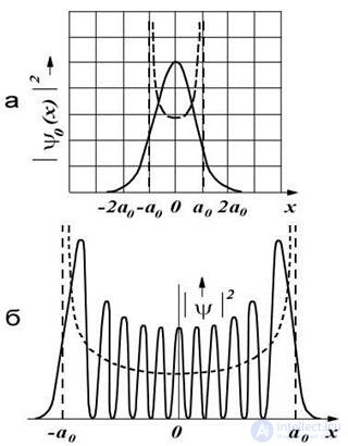
Fig. 4.11. Probability distributions for the classical (dashed) and quantum (solid line) oscillators.
a) n = 1; b) large values of n
Three-dimensional oscillator
This problem is a generalization of the preceding one. As with the three-dimensional potential well with infinitely high walls, the wave function is represented as a product of the wave functions of one-dimensional oscillators oscillating independently along the axes  ,
, ,
, . Thus, the ground-state wave function has the form
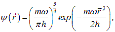
and the energy levels of the three-dimensional oscillator are described by the formula

Unlike the one-dimensional oscillator, the state is determined by the values of three quantum numbers 1, 2, 3. It is easy to see that all excited states must be degenerate.
N. Bohr, at the dawn of quantum mechanics, raised the question of its relation to classical mechanics. The ordinary energy values in our world are large compared with the characteristic energy of the ground state and the splitting of levels: from a high staircase we cannot make out the individual steps. Or, in the language of quantum mechanics: at large quantum numbers (high-lying levels) classical results should be reproduced. Let us show this using the example of the hydrogen atom.
In Sec. 3.1 the classical expression was obtained for the velocity of an electron in the Bohr atom on an orbit of radius R:
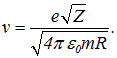
From this it is easy to obtain the classical frequency of revolution of the electron
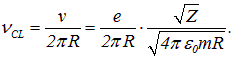
In addition, the classical expression was found for the energy of the electron on the orbit
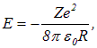
which allows the orbit radius to be expressed in terms of the electron energy
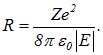
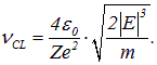
Substituting this expression into the formula for the classical frequency of revolution  , we obtain
|
|
|
(4.29) |
It is precisely at this frequency that radiation from the electron is expected in classical theory.
In addition, in the same section the expression was derived for the energy of the level with number  :
:
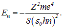
At  we obtain from this the quantum transition frequency
  between adjacent levels

Expressing the quantum number n in terms of the level energy, we find
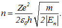
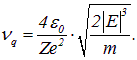
Substituting this expression into the formula for the quantum frequency of transition between adjacent high-lying levels, we arrive at the final result
|
|
|
(4.30) |
It is at this frequency that a strongly excited Bohr atom should radiate.
Comparing the classical frequency (4.29) with the quantum one (4.30), we see that for one and the same electron energy they coincide. This is characteristic not only of a hydrogen-like atom. An analogous result is obtained for an infinitely deep potential well, and the same conclusion can be drawn for other systems as well. Consequently, Bohr's correspondence principle holds:
|
Classical mechanics is the limiting case of quantum mechanics. |
Example. Using the formulas and data of the example from the previous section, let us demonstrate the validity of Bohr's correspondence principle for the translational motion of nitrogen molecules in a vessel.
When molecules transition between levels with an energy difference  a quantum of light is emitted with energy

from which we find
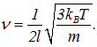
In addition, the classical velocity of nitrogen molecules equals

and they fly across the vessel from wall to wall and back in a time

(the period of classical motion). The reciprocal quantity is the classical frequency
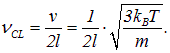
It is precisely at this frequency that classical physics predicts electromagnetic radiation. Thus, Bohr's correspondence principle manifests itself in the fact that both frequencies coincide — the quantum one (for transitions between highly excited states) and the classical one. The same holds, as we have seen, for the Bohr atom. If we substitute the numerical values, for the radiation frequency in this example we obtain the value

which corresponds to a wavelength
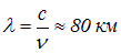
— extremely long radio waves.
Until now we have dealt with problems involving bound states. Let us now consider examples of infinite motion of particles, when they can move off to infinitely large distances. In the simplest case of motion along one of the coordinate axes, the problem of particle scattering reduces to the problem of the interaction of a particle with some potential barrier. We shall consider several types of barriers of simple rectangular shape, in order to bring out the characteristic features of this type of quantum phenomena.
Low infinite barrier
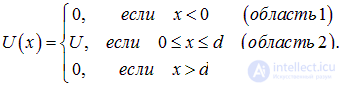
The potential energy has the form
|
|
|
(4.31) |
The word "low" means that the height of the barrier  is less than the energy of the particle
  (Fig. 4.12).
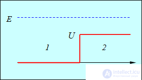
Fig. 4.12. Low potential barrier: the dashed line shows the energy of the particle incoming from the left,
the numbers — the numbers of the regions with different potential energy
Let us solve the Schrödinger equation separately for each of the regions. In region 1 the potential energy is zero, and we obtain the same equation (4.22) as for a free particle, with its general solution in the already familiar form
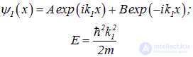
where  and
and  — are the amplitudes of the incident and reflected waves, respectively.
In region 2 the Schrödinger equation has the form

In this region the kinetic energy (and momentum) of the particle changes, and we must introduce a different wave vector (denote it  as opposed to the former
  )
)
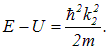
Then it is clear that the solution of the Schrödinger equation in region 2 will have the same form as for region 1 with  replaced by
  . However, from physical considerations it is clear that in region 2 there cannot be a wave propagating from right to left (at an infinitely distant point there is nothing for it to reflect from). Therefore the wave function in this region corresponds to a forward-traveling wave

In essence, here we again made use of a certain boundary condition, though a different one than for the bound-state problem. It remains only to determine the wave amplitudes  .
.
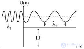
Fig. 4.13. Schematic form of the particle's wave function for the case of a low potential barrier
For this we must recall that  and
and  — are the values of one and the same wave function in different spatial regions. This wave function must be continuous together with its first derivative with respect to the variable x. Continuity of the function at the point x=0 means that the following condition must hold
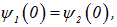
whence

Continuity of the first derivative of the wave function means the following equality must hold
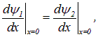
whence
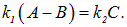
Solving the two equations obtained gives
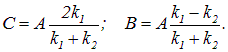
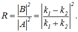
The amplitude of the incident wave remains undetermined: it is clear that it depends on the intensity of the particle flux! What matters is not the amplitudes themselves but the ratio R of the squares of their moduli, that is, of the intensities of the reflected and incident waves:
|
|
|
(4.32) |
The quantity R is called the reflection coefficient of the particle from the low barrier. In physical terms this is the probability of reflection of the particle from the barrier. Correspondingly, the quantity
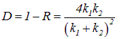 ,
,
called the transmission coefficient, determines the probability of the particle penetrating into the region on the right. It is remarkable that the particle has a chance of being reflected from a low barrier and turning back. In classical physics a particle always (R = 0) penetrates past the barrier, if it has enough energy to do so. For example, from the point of view of classical physics an electron with energy 10 eV, flying into a capacitor with a retarding field of 5 eV, would certainly overcome the retardation and continue on its way with a reduced energy of 5 eV. In quantum theory, however, the probability that the electron is reflected from the field of the capacitor and turns back is not zero. The reflection coefficient can be measured by directing a flux of particles at the barrier and measuring the fraction of particles reflected from it.
High infinite barrier
The potential energy has the same form, but the energy of the particle is less than the height of the barrier: <(Fig. 4.14).
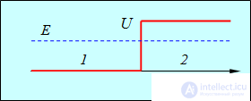
Fig. 4.14. High potential barrier
The solution in region 1 remains the same: a superposition of a forward and a reflected wave. In region 2, however, because of the reversed relation between the particle energy and the barrier height, the wave vector becomes imaginary:

where
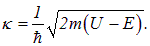
Substituting the imaginary wave vector

into expression (4.32) for the reflection coefficient R we obtain that R = 1. As in classical physics, a particle with energy less than the height of an infinite barrier will certainly be reflected from it. It is true that in classical physics the particle cannot penetrate under the barrier at all. Our solution of the Schrödinger equation for region 2 in the case of a high barrier becomes equal to

This is no longer a wave but an exponentially decaying function. As in the case of a low barrier, the unphysical solution — an exponentially growing function of the form

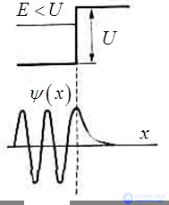
Fig. 4.15. Schematic form of the particle's wave function for the case of a high potential barrier
By the depth of penetration of the particle under the barrier  we mean the distance over which the intensity of the flux (probability) weakens by a factor of e. From the expression for
  it follows that

Potential barrier of finite width
The potential energy has the form
|
|
|
(4.33) |
It is clear what happens at >: with some probability the particle can be reflected from the barrier. The most interesting case is < (Fig. 4.16).
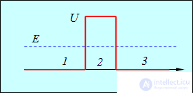
Fig. 4.16. Potential barrier of finite width
We saw that the intensity (square of the modulus of the amplitude) of the wave decreases under the barrier and at a distance becomes smaller by a factor of  . But at this point the barrier ends, so the wave will emerge freely to the right of the barrier with a reduced amplitude.
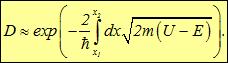
The ratio of the intensities of the outgoing and incident waves is called the transparency coefficient  (it is also equal to the probability of passage through the barrier). From the above reasoning follows an approximate expression for :
|
|
|
(4.34) |
In obtaining we dropped certain factors in front of the exponential, which physically means neglecting processes in which the particle, before leaving from under the barrier, undergoes multiple reflections from its walls. For a high and wide barrier  the contribution of such processes is small, and the approximation made is justified.
Penetration of a particle through a finite potential barrier is possible in quantum mechanics but is categorically forbidden in classical mechanics. Indeed, formally the quantity  plays the role of a (imaginary) momentum, so that the kinetic energy

becomes negative. The uncertainty relations save the day. The modulus of the (imaginary) velocity of the particle is of order

so that the tunneling time

The uncertainty in the kinetic energy
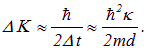
From the results obtained for the transparency coefficient it is seen that the tunneling effect is noticeable if

But then
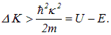
It turns out that the uncertainty in the kinetic energy of the particle under the barrier is greater than the value of the kinetic energy itself. Therefore it cannot be asserted that under the barrier the kinetic energy is negative. Rather, it is "smeared out" to such an extent that the particle can, as it were, leap over a not-too-large barrier. In the case of a high and wide barrier, on the other hand, the "smearing" of the kinetic energy must be very large, which is possible only for a very short time, during which the particle does not manage to slip through the barrier. Therefore in this case the transparency coefficient becomes exponentially small. Put differently: tunneling is noticeable when the barrier width is of the order of the de Broglie wavelength.
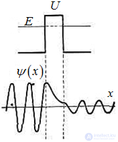
Fig. 4.17. Wave function of the particle for the case of a potential barrier of finite width
A barrier of arbitrary shape can be represented as a sequence of rectangular barriers; the theorem on the multiplication of probabilities leads to the appearance of a sum (integral) in the exponent, so that instead of (4.34) we have
|
|
|
(4.35) |
The integral is taken between the turning points

at which the classical particle must reverse its direction of motion.
Example 1. An electron is located in a one-dimensional potential well of width  (Fig. 4.18) and has energy
  . On one side of the well the potential energy
  is infinite, while on the other side a potential barrier of height
  and width
 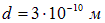 prevents the electron from leaving the well. Let us estimate the lifetime
  of the electron in the well.
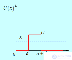
Fig. 4.18. A particle in a potential well formed by an impenetrable obstacle and a finite barrier
The velocity of the electron in the well

and in a time interval t it will approach the barrier

At each approach the probability of tunneling equals D, so that the probability of tunneling  over time t equals
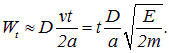
The probability  increases as the time interval t grows. At some value
  the tunneling probability will become equal to unity, and the electron will break free of the well. From this we obtain an estimate for the lifetime of the electron in the well:

It now remains to substitute the numerical data. To simplify the calculations it makes sense to calculate the transparency coefficient and the pre-exponential factor separately. We have

Now it remains to calculate the transparency coefficient:
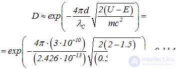
We finally obtain

Even by the standards of the microworld this time is small: before the electron seeps through the barrier, light manages to travel a distance of only 0.7 µm.
The transparency of the barrier depends strongly on the energy of the particle in the well and on the width and height of the barrier. For example, when the barrier width is doubled, the new transparency coefficient will, as is easy to guess, equal the square of the old one. For the electron this then gives a value of = 0.0013 and its lifetime in the well increases to  . This explains the absence of tunneling in the everyday world with its high and wide potential barriers.
Example 2. Let us solve the previous example, placing a proton instead of an electron in the same potential well.
To avoid solving an analogous problem from the very beginning, we can make use of the results of the previous example. The proton is more massive than the electron by a factor of 1837. In the transparency coefficient the mass of the particle enters under a square root in the exponent. When the mass changes by a factor of n, a factor appears in the exponent

and the new transparency coefficient will equal the old one raised to the power

Using the data of the previous example, we obtain

The pre-exponential factor will also be multiplied by

and the lifetime of the proton in the potential well will equal

This turns out to be such a huge quantity that the proton would live in the well forever: the age of the Universe is "only"  .
.
These two problems demonstrate the strong dependence of barrier permeability on the mass of the particle.
In this section we shall show that the passage of a quantum particle through a low potential barrier is analogous to the reflection of light at the boundary of two half-infinite media. Further, the passage of a particle through a potential barrier of finite width can be described as multiple reflection of classical waves, and as a result we again arrive at well-known results of optics. The purpose of this section is to demonstrate the close connection between different branches of physics.
Step potential
We again depict this potential in Fig. 4.19.
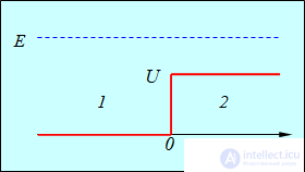
Fig. 4.19. Passage of a particle over a step barrier:
the process is equivalent to normal incidence of light from vacuum (1)
onto a half-infinite medium (2) with refractive index

Establishing an analogy between quantum mechanics and light means that we want to find such replacements of the quantum-mechanical characteristics of the particle's motion by the characteristics of light that the formulas of quantum mechanics turn into the corresponding formulas for the propagation of light. The replacement procedure will be depicted in the formulas by double arrows, with the quantum-mechanical quantities on the left and the optical ones on the right. These formulas should be distinguished from equalities in which quantities on both sides refer either to the particle or to the light wave.
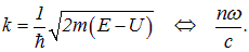
The propagation of a quantum particle is described in terms of its wave vector

where

is the kinetic energy of the particle. Here and below we write the formulas for the particle referring to the barrier region; the relations for the particle outside the barrier are obtained at  = 0. The velocity of the particle is given by the relation
|
|
|
(4.36) |
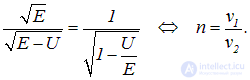
Let us first introduce the refractive index  of medium 2, corresponding to the barrier region: it is natural to define it as the ratio of the particle's velocities in regions 1 and 2 (we take the refractive index in region 1 to equal unity, as in vacuum, that is,
  )
)
|
|
|
(4.37) |
At = 0 we obtain n = 1 — the refractive index of vacuum.
The wave vector of a light wave is related to the angular frequency by

We shall also assume that the particle's wave vector, under the sought replacement, turns into the wave vector of light, that is
|
|
|
(4.38) |
From the relation

for a medium without dispersion it follows that the group velocity of light is

into which, under the sought replacement, the velocity of the particle  must turn. Then equation (4.36) gives
|
|
|
(4.39) |
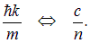
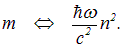
Dividing equation (4.38) by (4.39), we find yet another replacement
|
|
|
(4.40) |
Of course, the "mass" standing here on the left side cannot be identified with the mass of the photon, which equals zero. We can call it the "effective mass of the photon." In vacuum, at n = 1, it equals

This quantity corresponds to the well-known relativistic mass—energy relation, and it arises in the study of the influence of a gravitational field on the propagation of light.
Be that as it may, the point is that these replacements, as we shall see, translate the formulas of quantum mechanics into the formulas of optics.
Considering the passage of a particle over a low potential barrier (see the step potential in Fig. 4.19), we have already derived the transmission coefficient, which we denote here by  :
:
|
|
|
(4.41) |
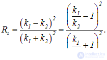
The reflection coefficient (30.32), equal to  , we rewrite in the form
|
|
|
(4.42) |
Applying the replacements given above, which in this case reduce to the replacement

we write the corresponding transmission and reflection coefficients for light incident perpendicularly from vacuum onto a medium with refractive index :
|
|
|
(4.43) |
In optics precisely such formulas are called the Fresnel formulas for the relative intensity of reflected and refracted light at an angle of incidence of 90°. We are once again convinced that physics (or nature) is unified, and that quantum mechanics has deep roots not only in classical mechanics but also in wave optics.
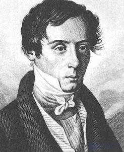
Fig. 4.20. Augustin-Jean Fresnel (1788–1827)
Rectangular barrier of finite width
The potential barrier is shown in Fig. 4.21.
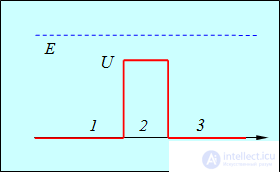
Fig. 4.21. Passage of a particle over a finite rectangular barrier:
the process is equivalent to multiple reflections from the barrier shown in Fig. 4.19
The problem can be solved in the standard way, by writing the superposition of plane waves for each of the three regions 1, 2, and 3 and then matching the solutions to find the wave amplitudes. However, we shall replace this routine method with a classical treatment of the passage of waves, which will allow us to reveal the physical meaning of the resulting outcome.
Let us note first of all that a finite barrier can be regarded as a superposition of two step barriers, located at the points  and
and  . This remark makes it possible to use the formulas obtained earlier.
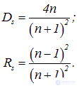
Let a de Broglie wave with amplitude equal to unity travel from left to right and enter the region above the barrier at the point . Owing to partial reflection its amplitude decreases and becomes equal to

where  — is the transparency coefficient of the step barrier. It then propagates to the point , acquiring along the way a phase shift
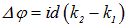
compared with the phase of a free particle at the same point. Here the wave once again encounters a step barrier, as a result of which its amplitude again decreases to the value

As a result the wave will emerge beyond the barrier with an amplitude
|
|
|
(4.44) |
But we have accounted for only part of the wave emerging outward. The wave that arrives at the point is partially reflected from it (an additional factor

in the amplitude), travels back to the point , is reflected there again (a factor

in the amplitude), returns back to the point , where it finally emerges outward. The total path traveled by this part of the wave equals 3d, giving a phase shift

As a result this part of the wave will emerge beyond the barrier with amplitude
|
|
|
(4.45) |
In a similar way processes with 2n reflections inside the barrier occur, and each of them leads to a wave with amplitude
|
|
|
(4.46) |
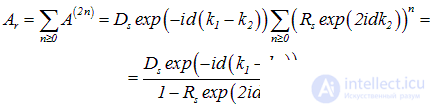
The amplitude  of the resultant wave is obtained by summing expression (4.46) over all n from zero to infinity:
|
|
|
(4.47) |
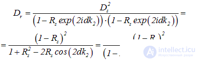
The modulus of the amplitude  of the wave that has passed over the barrier gives us the transmission coefficient
|
|
|
(4.48) |
Substituting here the quantum-mechanical expression (4.42) for  , we obtain
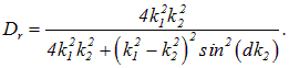
|
|
|
(4.49) |
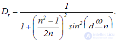
The standard solution of the Schrödinger equation gives exactly the same result. Passing over to optics, we replace  by expression (4.43) and
  — by
— by  . We then obtain the transparency coefficient of a plate of finite thickness
  for normal incidence of light with frequency
  :
:
|
|
|
(4.50) |
This expression also exactly reproduces the result of wave optics.
In a similar manner one can consider the wave reflected from the barrier, but the result is already known to us: the reflection coefficient from the finite barrier can be calculated using the formula

Studying formulas (4.49) and (4.50), we discover "windows of transparency" at certain values of the frequency of the incident light, when 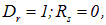 that is, there is no reflected wave at all. This happens when

that is, when an even number of half-waves (or a whole number of waves) of light in the medium fits into the double width of the barrier:

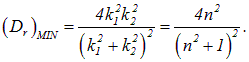
In the opposite case, when the double width of the barrier equals an odd number of half-waves

we arrive at the minimum value of the transparency coefficient
|
|
|
(4.51) |
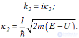
In the case  we are dealing with tunneling — the particle "moves" inside the barrier with an "imaginary" wave vector
|
|
|
(4.52) |
In this case the trigonometric function turns into a hyperbolic one
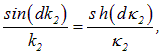
and from
продолжение следует...
Часть 1 4. The Schrodinger equation
Часть 2 4.6. Bohr's correspondence principle - 4. The Schrodinger equation
Часть 3 - 4. The Schrodinger equation







Comments