
Lecture
Это окончание невероятной информации про постоянный электрический ток.
...
disconnected.
|
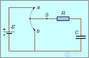
Fig. 4.20. Circuit for charging and discharging a capacitor Suppose the capacitor of capacitance C is initially uncharged, and we flip the switch to position a. A time-dependent current I(t) will flow through the circuit, carrying positive charge onto the upper plate of the capacitor. Note that although the charging and discharging current of the capacitor is not constant, it is considered here because its variation in this case can be regarded as slow. Let us denote the charge on this plate at time t by q(t). The voltage across the capacitor can be found as the difference between the emf and the voltage drop across the load, that is,
According to the law of conservation of charge, the change in the charge q on the capacitor plates occurs only because of the presence of the current I. Therefore the second equation of the process has the form
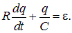
Substituting (4.37) into (4.36):
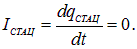
We see that this equation has a stationary solution (constant charge on the capacitor)
At such a charge on the capacitor, the voltage across it equals the emf of the current source, and no current flows in the circuit Let us introduce the deviation of the charge on the capacitor from its stationary value
or
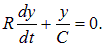
Substituting this relation into (4.38), we find the equation for the function y(t)
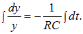
This equation is easily integrated
whence
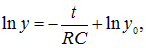
Evaluating the integrals, we find
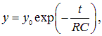
or
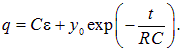
where y0 — is an arbitrary constant of integration (the value of y at the initial instant of time). From this we find the charge on the capacitor
It remains for us to use the initial condition: at the instant t = 0 the capacitor was uncharged
From this we find
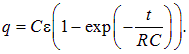
and finally
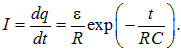
Differentiating q(t) with respect to time, we find the current in the circuit |
|
|
(4.40) |
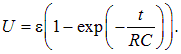
The voltage across the capacitor U(t) = q(t)/C is readily obtained from (4.39)
|
|
(4.41) |
Thus, as the charge and voltage on the capacitor grow, the current in the circuit decreases. In this case the charge of the capacitor tends to its stationary value  and the voltage across the capacitor tends to the emf of the current source. The quantity
  has the dimension of time and determines the characteristic time of the charging process. Over the interval
  the current in the circuit decreases
by a factor of e = 2.72.
Fig. 4.21 shows the dependence of the charge on the capacitor and the current in the circuit for specific values R = 1.5 kΩ, C = 2 μF,  The characteristic time of the process for these values equals
  It can be seen from the graphs that already at times of order

the capacitor is almost fully charged.
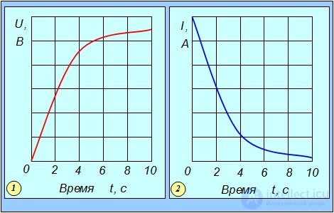
Fig. 4.21. Graphs of the voltage across the capacitor (left) and the current in the circuit (right)
during the charging of a capacitor of capacitance C = 2 μF through an active resistance R = 1.5 kΩ from a current source with emf 12 V
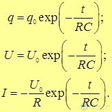
Let us now consider the process of discharging a capacitor. Having charged it to some charge  (or, equivalently, to an initial voltage U0 = q0/C), we flip the switch to position b (see Fig. 4.20). The capacitor will begin to discharge, and a current will flow through the circuit. We have the same equations except that no current source is included in the circuit. Therefore in this case we must set
  in equation (4.38). Then it coincides with what we solved earlier for y(t), so the solutions for the capacitor discharging process are already known to us
|
|
(4.42) |
All these quantities decrease rapidly with time: over the same characteristic interval  the charge of the capacitor, the voltage across it, and the current in the circuit drop by a factor of 2.72. The negative sign in the expression for the current means that during discharge the current flows in the direction opposite to the current during charging of the capacitor.
In practice, complex (branched) electric circuits are very often encountered, for the calculation of which it is convenient to use Kirchhoff's rules (Fig. 4.22).
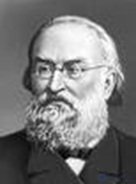
Fig. 4.22. G. Kirchhoff (1824–1887) — German physicist
Kirchhoff's first rule is a consequence of the law of conservation of charge and of the natural requirement that in stationary processes charge should not accumulate or decrease at any point of a conductor. This rule applies to nodes, that is, to those points in a branched circuit at which at least three conductors meet.
Kirchhoff's first rule states:
|
The algebraic sum of the currents meeting at a node is zero, that is, the amount of charge arriving at a given point of the circuit per unit time equals the amount of charge leaving that point in the same time
|
Here the currents flowing toward a node and away from it have opposite signs (Fig. 4.23).
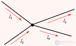
Fig. 4.23. The sum of the currents meeting at a node is zero
Kirchhoff's second rule is a generalization of Ohm's law and applies to any closed loop of a branched circuit.
Kirchhoff's second rule states:
|
In any closed loop of a circuit, the algebraic sum of the products of the currents and the resistances of the corresponding sections of the loop equals the algebraic sum of the emfs in the loop (Fig. 4.24)
|
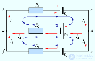
Fig. 4.24. Example of a branched electric circuit.
The circuit contains one independent node (a or d) and two independent loops (for example, abcd and adef)
Kirchhoff's rules make it possible to determine the magnitude and direction of the current in any part of a branched circuit, provided the resistances of its sections and the emfs included in them are known. The number of equations written from Kirchhoff's first and second rules must equal the number of unknown quantities sought. Using the first rule for a branched circuit containing m nodes and n branches (sections), one can write (m – 1) independent equations, and using the second rule, (n – m + 1) independent equations.
Let us give an example of calculating the currents in a branched circuit (Fig. 4.25).
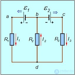
Fig. 4.25. Example of a branched circuit
The directions of the emfs are shown by blue arrows. In this circuit we have two nodes — points b and d (m = 2), and three branches — the section b–a–d with current I1, the section b–d with current I2, and the section b–c–d with current I3 (n = 3). Hence, we can write one (m – 1 = 2 – 1 = 1) equation from the first rule and two (n – m + 1 = 3 – 2 + 1 = 2) equations from the second rule. How is this done in practice?
Step one. Let us choose directions for the currents flowing in each of the branches of the circuit. It is entirely unimportant how these directions are chosen. If we guessed correctly, the value of this current will come out positive in the final result; if not, and the direction should have been reversed, the value of this current will come out negative. In our example we chose the current directions as shown in the figure. It is important to stress that the directions of the emfs are not arbitrary — they are determined by the way the poles of the current sources are connected (see Fig. 4.25).
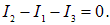
Step two. We write Kirchhoff's first rule for all nodes except one (at the last node, whose choice is arbitrary, this rule will be satisfied automatically). In our case we can write the equation for node b, into which current I2 flows and out of which currents I1 and I3 flow
|
|
(4.45) |
Step three. It remains for us to write the equations (in our case – two) for the second rule. To do this we need to choose two independent closed loops. In the example under consideration there are three such possibilities: the path around the left loop b–a–d–b, the path around the right loop b–c–d–b, and the path around the whole circuit b–a–d–c–b. It is enough to take any two of them, and then the second rule will be satisfied automatically for the third loop. The direction of traversal of the loop does not matter, but during traversal a current is taken with a plus sign if it flows in the direction of traversal, and with a minus sign if it flows in the opposite direction. The same applies to the signs of the emfs.
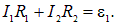
Let us first take the loop b–a–d–b. We start from point b and move counterclockwise. Along our path we meet two currents, I1 and I2, whose directions coincide with the chosen direction of traversal. The emf  also acts in this same direction. Therefore the second rule for this part of the circuit is written as
|
|
(4.46) |
As the second closed path, for variety let us choose the path b–a–d–c–b around the whole circuit. Along this path we meet two currents I1 and I3, of which the first enters with a plus sign and the second — with a minus sign. We also meet two emfs, of which  enters the equation with a plus sign, and
  — with a minus sign. The equation for this closed path has the form
|
|
(4.47) |
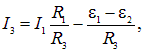
Step four. We have found three equations for the three unknown currents in the circuit. The solution of an arbitrary system of linear equations is described in a course of mathematics. For our purposes (the circuit is simple enough) we can simply express I3 in terms of I1 from equation (4.47)
|
|
(4.48) |
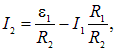
I2 in terms of I1 by means of equation (4.46)
|
|
(4.49) |
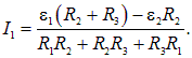
and substitute (4.48), (4.49) into the equation of the first rule (4.45). This equation contains only the unknown I1, which is found without difficulty
|
|
(4.50) |
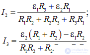
Substituting this expression into (4.48), (4.49), we find respectively the currents I2, I3
|
|
(4.51) |
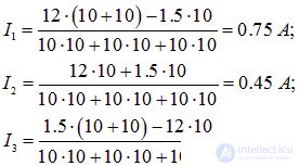
Step five. Numerical values, once given, are substituted into the formulas found. Let us calculate, as an example, the currents in our circuit for equal resistances R1 = R2 = R3 = 10 Ω, but different emfs  We have:
|
|
(4.52) |
The last value came out negative for the given numerical parameters of the circuit. This means that in reality the current direction is opposite to that shown in the figure. This is natural: the powerful left source sends out a current of 0.75 A, part of which (0.45 A) branches off into the middle branch, while the remainder — 0.3 A — continues to flow in the same direction, which the low-power right battery cannot prevent.
Note. Kirchhoff's rules make it possible, in principle, to calculate circuits of any complexity. But the calculations can be quite complicated. Therefore it is recommended first to look for possible symmetry of the circuit. Sometimes it is more or less obvious from symmetry considerations that certain currents are equal to each other or certain voltages are equal to zero (in which case the corresponding section of the circuit can be excluded from consideration). If this is possible, the calculations are considerably simplified.
In our example we neglected the internal resistance of the current sources. If it is present, it must also be included in the equations of the second rule.
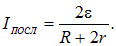
Example. Two identical current sources with emf  and internal resistance r are combined into a battery. Two connection options are possible — series and parallel (Fig. 4.26). With which connection will the current in the load R be largest?
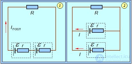
Fig. 4.26. Series (1) and parallel (2) connection of current sources
Solution. The calculation is especially simple for the series connection: there is no equation from the first rule, since there are no nodes in the circuit. The single equation of the second rule gives
|
|
(4.53) |
To simplify the calculation of the parallel connection, let us take into account that, from symmetry considerations, the currents through the sources must be equal and coincide in direction. Then the first rule gives
|
|
(4.54) |
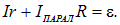
Kirchhoff's second rule, written for the path through the lower source and the load, has the form
|
|
(4.55) |
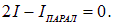
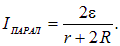
From this it follows that
|
|
(4.56) |
Comparing (4.53) and (4.56), we find that for R > r the series battery's current is greater (Iseries > Iparallel), while for R < r it is smaller (Iseries < Iparallel) than the current from the parallel battery. When the internal resistance equals the load, R = r, both batteries give the same current.
Suppose that at the ends of a section of conductor there is a potential difference 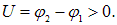 Moving from point 2 at higher potential to point 1, where the potential is lower, a positive charge
  loses energy

By definition, for direct current

then

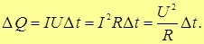
and the energy lost (or the work done by the electric field forces) equals

Where does this energy go? It does not turn into kinetic energy of the charge, since at constant current the drift velocity of the charges is unchanged. Recall that the charge is not accelerated because of collisions with the atoms of the conductor's crystal lattice. So, if a current flows through a conductor and the conductor is stationary, the work done by the electric field forces is spent heating the conductor. Colliding with the particles of the conductor, the charge carrier transfers to them the energy it receives from the field. Hence the work done by the field on the charges ultimately turns into the energy of the thermal (chaotic) motion of the atoms of the conductor, that is, the conductor heats up (Figs. 27, 28, 29).

Fig. 4.27. Release of heat in an electric discharge
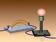
Fig. 4.28. Release of heat in a resistor and an incandescent lamp
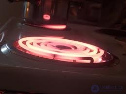
Fig. 4.29. Release of heat in a heating element
Video 4.7. Release of heat in series-connected conductors of different resistivity.
Thus, the work A done over time  is released in the conductor as heat
|
|
(4.57) |
This formula is called the Joule–Lenz law. The law was established by J. Joule in 1841 (Fig. 4.30) and, independently of him, by the Russian physicist E.Kh. Lenz in 1842.
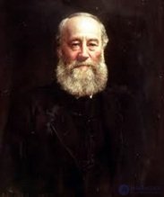
Fig. 4.30. J. Joule (1818–1889) — English physicist
Example. Suppose a capacitor of capacitance C, charged to a potential difference U, discharges through a resistance R. Find the total amount of heat released in the load (Fig. 4.31).
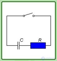
Fig. 4.31. Electric circuit with a charged capacitor and a resistance
Solution. In (4.42) we found the discharge current as a function of time. Substituting it into (4.57) and integrating over t.
As should be expected, all of the electric field energy originally stored in the capacitor turned into heat.
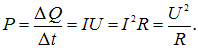
The amount of heat released per unit time (that is, the thermal power P) equals
|
|
(4.58) |
Heat is released throughout the volume of the conductor. Let us find the density of the thermal power, that is, the power released per unit volume. Imagine a linear conductor of constant cross-section S and length l. Then the voltage across the ends of the conductor can be expressed in terms of the electric field strength within it

On the other hand, the resistance of the conductor equals

(recall that  — is the conductivity of the given substance, the reciprocal of its resistivity
  ). From this we find
|
|
(4.59) |
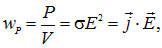
Thus, the density of the thermal power equals
|
|
(4.60) |
where j — is the current density. We derived this formula for a linear conductor, but it is also valid in the general case. For conductors of complex shape or composed of different materials, the heat released per unit time can be calculated by integrating the thermal power density over the whole volume of the conductor
|
|
(4.61) |
Fig. 4.32 shows an experiment demonstrating the distribution of power between series- and parallel-connected conductors of different resistance. For this, two lamps are connected into a circuit with a voltage of 40 V, whose power ratings are 25 W and 150 W when a voltage of 127 V is applied to them. When these lamps are connected in series, only the filament of the lower-power lamp, which has the higher resistance, glows, while when connected in parallel, the higher-power lamp, which has the lower resistance, glows more brightly.
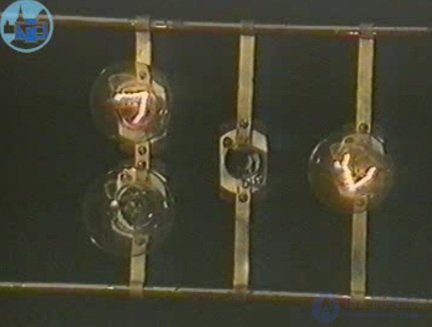
Fig. 4.32. Distribution of power between series- and parallel-connected conductors
At the beginning of the twentieth century it was proven experimentally that free electrons are the charge carriers in metals. Proceeding from these concepts, the German physicist Drude created (1900) the classical electron theory of metallic conductivity, later improved by other physicists. The internal structure of metals is characterized by a crystal lattice, such as, for example, the one shown in (Fig. 4.33).
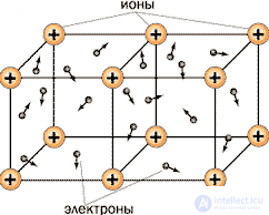
Fig. 4.33. Diagram of the crystal lattice of metals
Positive ions, which are metal atoms stripped of one or several valence electrons and therefore positively charged, are located at the sites of the lattice. These positive ions are capable of only small thermal oscillations about their equilibrium positions at the lattice sites. In the space between the ions, the valence electrons, torn away from the atoms and «shared» by the crystal, move practically freely, forming what is called the electron gas. According to Drude's theory, the electrons in the crystal lattice behave in many respects like an ideal gas, so the well-known formulas of the kinetic theory of gases can be used to describe their behavior (Fig. 4.34).
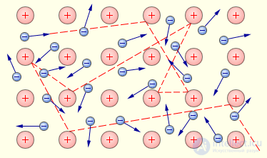
Fig. 4.34. Gas of free electrons in the crystal lattice of a metal.
The trajectory of one of the electrons is shown
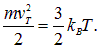
In the absence of an external field, all directions of the velocity of electrons in chaotic thermal motion are equally probable; consequently, the average current density is zero, and one can say that the electron gas as a whole is at rest relative to the positive ions of the lattice. According to classical thermodynamics, the average energy of the translational thermal motion of the molecules of any gas depends only on the temperature T, but not on the chemical nature or molecular weight of the gas, and equals
|
|
(4.62) |
From this we find the root-mean-square velocity of the chaotic motion of the particles
|
|
(4.63) |
Remark: Note that relations (4.62), (4.63) and those following from them hold only when the distribution of the particles (in this case, electrons) over velocities is Maxwellian, which in turn is the case when the translational motion is entirely classical. The electron gas in a metal is a quantum system and is not described by the Maxwell distribution. Therefore the presentation of the classical Drude theory undertaken below is of limited interest, as a way of obtaining relations that are qualitatively (dimensionally) correct but cannot in any way claim quantitative agreement with experiment.
We saw (see Sec. 4.1) that for room temperatures vT = 106 m/s. When an external electric field is present, the electrons in the metal will also possess some average (drift) velocity v of directed motion against the external field E. According to the estimates given above, the velocity v is many orders of magnitude smaller than the velocity vT (Fig. 4.35).
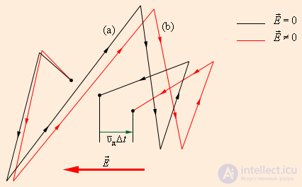
Fig. 4.35. Motion of a free electron in a crystal lattice:
a — chaotic motion of an electron in the crystal lattice of a metal;
b — chaotic motion with a drift caused by the electric field.
The scale of the drift is greatly exaggerated
If the electron gas in a metal is treated as an ideal gas, then the thermal motion of the electrons in the crystal lattice can be characterized by the mean free path  , that is, the average distance traveled by freely moving electrons in the metal between two successive collisions with lattice ions. The average time between two collisions will be

Since v << vT, we can assume that neither  nor changes when an electric field E is applied.
Ohm's law
When an external electric field E is present, a force F = eE acts on the electron, as a result of which it acquires an acceleration

(m — the mass of the electron). Let us assume that upon colliding with an ion, the electron completely loses its directed-motion velocity: vmin = 0. It then begins to accelerate under the electric field and by the next collision acquires a velocity
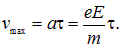
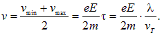
Consequently, the average velocity of directed motion v over the period between two collisions, that is, over the time is
|
|
(4.64) |
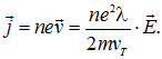
Hence the current density will be equal to
|
|
(4.65) |
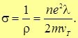
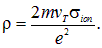
Comparing the resulting expression for the current density j with Ohm's law (4.9), we obtain the formula for the conductivity s and for the associated resistivity 
|
|
(4.66) |
Let us give some numerical estimates. As will be shown further on, the relation between the mean free path and the effective
cross-section  of the scattering center (ion) and the concentration of these centers has the form

For metals, as we have already discussed, the concentration of ions approximately coincides with the concentration of free electrons

Substituting the expression for  into formula (4.66), we obtain
|
|
(4.67) |
An estimate for the cross-section can be obtained knowing the order of magnitude of atomic diameters

whence
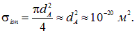
The velocity of chaotic motion was estimated as vT = 105 m/s. We now obtain from (4.67) the value of the resistivity
|
|
(4.68) |
The estimate obtained does indeed reproduce the order of magnitude of the resistivities of metals given in the table (see Sec. 4.3).
The Joule–Lenz law
Upon colliding with an ion, as we assumed, the electron transfers to it the drift energy it has accumulated over the time 
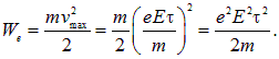
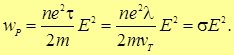
Multiplying We by the electron concentration n and dividing by the time  we obtain the thermal energy transferred to a unit volume of the conductor per unit time (that is, the power density)
|
|
(4.69) |
The last equality in this chain is obtained using expression (14.66) for  . As a result, we have derived the Joule–Lenz law (4.60) from the microscopic theory.
The Wiedemann–Franz law
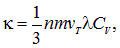
Metals, along with high electrical conductivity, are also characterized by high thermal conductivity. In 1853, the German physicists G. Wiedemann and R. Franz established an empirical law, according to which the ratio of the thermal conductivity coefficient k to the electrical conductivity coefficient s is approximately the same for all metals and varies proportionally to temperature. The thermal conductivity of metals significantly exceeds the thermal conductivity of dielectrics, from which one can conclude that thermal conductivity in metals is mainly due to the electron gas rather than to its crystal lattice. For the thermal conductivity coefficient of the electron gas in a metal, an expression can be borrowed from the kinetic theory of gases
|
|
(4.70) |
where the product nm of the electron concentration and their mass is substituted in place of the density of the electron gas.
The specific heat capacity of a monatomic gas equals
|
|
(4.71) |
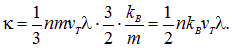
Substituting this value into the expression for the thermal conductivity coefficient k, we obtain
|
|
(4.72) |
Dividing k by  , we obtain
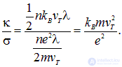
Since
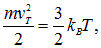
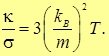
we arrive at the relation
|
|
(4.73) |
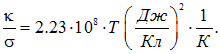
This relation expresses the Wiedemann–Franz law. Substituting the values kB = 1.38·10–23 J/K and e = 1.6·10–19 C, we obtain
|
|
(4.74) |
However, the relation obtained does not agree sufficiently accurately with experiment, that is, the classical theory explained the Wiedemann–Franz law only qualitatively. The dependence of resistivity on temperature that follows from the classical theory
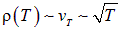
also does not agree with experiment. Only quantum theory was able to explain all the discrepancies.
The relation between the directed-motion velocity  and the charge-flux-density vector (current density)
  and the electric field strength can be obtained within the framework of the following, sufficiently simple, phenomenological model. When an electron collides with a heavy ion of the crystal lattice (for example, for aluminum
 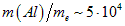 ) the electron loses practically all of its directed-motion momentum. According to Newton's second law, the rate of change of momentum equals the force acting on the body. Since collisions of electrons with ions lead to a loss of momentum, it is natural, firstly, to call this force a friction force. Secondly, the greater the electron's velocity before the collision, the greater the momentum it will lose, so this friction force must be proportional to the directed-motion velocity of the electrons. Let us write it in the form
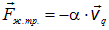 ,
,
then the equation of directed motion of the electron — the equation of Newton's second law for this motion under the action of an electric field of strength  has the form
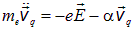
We are looking for a stationary solution corresponding to a constant current, when the directed-motion velocity  and
and  . In this case it follows directly from the previous relation that
 .
.
The minus sign in this relation is due to the fact that the electron is negatively charged. For the current density we immediately obtain:

It should be noted that the result does not depend on the sign of the charge carrier.
Часть 1 Direct electric current: current, voltage, emf, laws and rules
Часть 2 4.5. Kirchhoff's rules - Direct electric current: current, voltage, emf,
 or as the ratio of the charge to the capacitance q/C. Equating these expressions, we obtain the first equation of the charging process
















Comments