5.2 Amplitude Modulation

In the process of amplitude modulation, the amplitude U _{0 of the} carrying col u *** (u) = U ₀ cos (ωt + φ) ceases to be constant and changes according to the law of the transmitted message. The amplitude U (t) of the carrying noise *** can be related to the transmitted message:

U (t) = U ₀ + k _A e (t), (5.1)

where U ₀ is the amplitude of the carrier ring *** in the absence of a message (unmodulated ring ***); e (t) is a time-dependent function corresponding to the transmitted message (it is called a modulating signal); k _A is the proportionality coefficient reflecting the degree of influence of the modulating signal on the magnitude of the change in the amplitude of the resulting signal (modulated colo ***).

The expression for the amplitude-modulated signal in the general case is:

u _AM (t) = [U ₀ + k _A e (t)] cos (ω ₀ t + φ). (5.2)

The simplest case for the analysis is the case of an amplitude-modulated *** collation obtained if the harmonic collation *** is used as the modulating signal (such a case is called tone modulation):

e (t) = E cos (´Ωt + Θ), (5.3)

where Е is the amplitude, ´Ω is the angular frequency; Θ - the initial phase of the modulating signal.

To simplify the analysis, we will assume that the initial phases of a collar *** are zero, which does not affect the generality of conclusions. Then for tonal amplitude modulation you can write:

u _AM (t) = [U ₀ + k _A E cos´Ωt] cosω ₀ t = U ₀ [1+ M _A cos´Ωt] cosω ₀ t, (5.4)

where M _A = Е / U ₀ is the amplitude modulation coefficient (sometimes it is said - the depth of amplitude modulation).

To determine the spectrum of an amplitude-modulated colossus ***, we perform simple transformations of expression (5.4):

u _AM (t) = U ₀ cos ω ₀ t + U ₀ M _A cos ´Ωt cos ω ₀ t = U ₀ cos ω ₀ t + (U ₀ M _A / 2) cos (ω ₀ - ´Ω) t + (U ₀ M _A / 2) cos (ω ₀ + ´Ω) t. (5.5)

From the analysis of expression (5.5), it follows that with amplitude modulation by a harmonic colour ***, the spectrum of the amplitude-modulated signal contains three harmonic components. The harmonic component with frequency ω ₀ is the original unmodulated carrier with frequency ω ₀ and amplitude U ₀ .

Harmonic components with frequencies equal to (ω ₀ - ´Ω) and (ω ₀ + ´Ω) are the product of amplitude modulation and are called, respectively, the lower and upper lateral components. The amplitudes of the side components are the same, equal to U ₀ M _A / 2 and are located symmetrically with respect to the carrier frequency ω ₀ at a distance equal to - ´Ω. Thus, the width of the frequency band Δω occupied by the amplitude-modulated collar *** when modulated by a harmonic signal with a frequency ´Ω is equal to Δω = 2´Ω.

Graphs of the carrier range of *** u ₀ (t), modulating signal e (t) and amplitude-modulated signal u _AM (t) are shown in Figure 5.1.

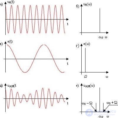
Fig. 5.1 Tonal amplitude modulation:
a) the carrying ring *** and its spectrum (b);
c) the modulating signal and its spectrum (d);
e) amplitude-modulated colony *** and its spectrum (e)

In the absence of modulation (M _A = 0), the amplitudes of the lateral components are zero and the spectrum of the amplitude-modulated signal consists only of a carrier collar *** with a frequency ω ₀ . When the amplitude modulation factor M _A <1, the amplitude of the resulting colossus *** changes from the maximum value U _MAX = U ₀ (1 + M _A ) to the minimum U _MIN = U ₀ (1 - M _A ).

Thus, the amplitude modulation factor M _A can be defined as

M _A = (U _MAX - U _MIN ) / (U _MAX + U _MIN ). (5.6)

When the amplitude modulation factor M _A > 1, distortions arise, called overmodulation (Figure 5.2). Such distortions can lead to loss of information and try to prevent them.

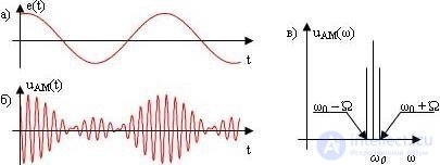
Fig. 5.2 Tonal amplitude modulation with the coefficient M _A > 1:
a) modulating signal; b) amplitude-modulated colony *** and its spectrum (c)

A similar approach can be applied to the analysis of amplitude-modulated complex *** complex shapes. In this case, the periodic modulating signal can be represented by a set of harmonic components whose frequency is a multiple of the period of the original signal. Each of the harmonics of the modulating signal in the spectrum of the amplitude-modulated colony *** of the two side components symmetrically separated from the carrier by an amount equal to the frequency of the corresponding harmonic. For example, if the spectrum of the modulating signal has the form shown in Fig. 5.3, a, then the spectrum of the amplitude-modulated colony *** can be represented by the diagram shown in Fig. 5.3, b.

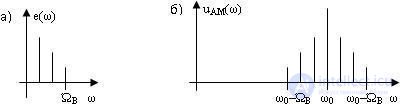
Fig. 5.3 Spectra of signals: a) modulating signal; b) amplitude modulated col ***

In the general case, the width P _{AM of the} spectrum of an amplitude-modulated col *** is equal to

P _AM = 2 Ω _B , (5.7)

where ´Ω is the upper (highest) frequency in the spectrum of the modulating signal.

Amplitude modulation is a type of modulation in which the variable parameter of the carrier signal is its amplitude

Application in radio engineering

The first experience of transmitting speech and music by radio using the amplitude modulation method was made in 1906 by an American engineer. Fessenden. The carrier frequency of the 50 kHz radio transmitter was developed by a machine generator (alternator), to modulate it between the generator and the antenna, a carbon microphone was switched on, changing the signal attenuation in the circuit. From 1920, instead of alternators, electron tube generators were used. In the second half of the 1930s, as the development of ultrashort waves, amplitude modulation gradually began to be crowded out of broadcasting and radio communications on VHF frequency modulation. From the middle of the 20th century, a single sideband modulation, which has a number of important advantages over AM, has been introduced in office and amateur radio communications at all frequencies. The question of transferring to OBP and broadcasting was raised, however, this would require replacing all broadcasting receivers with more complex and expensive ones, therefore it was not implemented. At the end of the 20th century, the transition to digital broadcasting began using signals with amplitude shift keying. ^[one]

Definition

Let be

• - information signal, ,
• - bearing ring ***.

Then the amplitude modulated signal can be written as follows:

Here - some constant called modulation factor. Formula (1) describes the carrier signal amplitude modulated signal with modulation factor . It is also assumed that the following conditions are met:

The fulfillment of conditions (2) is necessary so that the expression in square brackets in (1) is always positive. If it can take on negative values ​​at some point in time, then so-called overmodulation (redundant modulation) occurs. Simple demodulators (such as a quadratic detector) demodulate such a signal with strong distortions.

Example

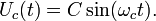
Suppose that we want to modulate the ring carrying *** monoharmonic signal. The expression for the carrier case with frequency , the initial phase is set equal to zero, has the form

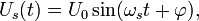
Expression for a modulating sinusoidal signal with a frequency has the appearance

Where - the initial phase. Then, in accordance with (1)

The above formula for can be written as follows:

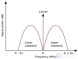
The radio signal consists of a carrier ring *** and two sinusoidal columns ***, called sidebands, each of which has a frequency different from . For the sine wave used here, the frequencies are and . As long as the carrier frequencies of neighboring radio stations are quite separated, and the sidebands do not overlap with each other, the stations will not influence each other.