
Lecture
A cylindrical wave is a model of a wave process, a wave radially diverging from some line in space or converging toward it. A special case of a cylindrical wave in a plane is a circular wave, diverging from a point (or converging toward it).
Generally speaking, an electromagnetic field cannot be obtained from a single
scalar function depending on a point and time; because of this, the analysis of
electromagnetic fields is by its very nature more complex than the study of
heat flows or the transmission of acoustic oscillations. In the three-dimensional
scalar wave equation, the variables separate in 11 different coordinate
systems ^), but complete solutions of the vector wave equation in a form
directly applicable to solving boundary-value problems are known at the
present time only for certain separable systems of cylindrical
coordinates and for spherical coordinates. As will be shown, in such
systems the electromagnetic field can be decomposed into two field components,
each of which is obtained from
a single scalar function
satisfying the wave equation.
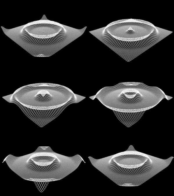
The front of a cylindrical wave is a cylindrical surface, on whose axis lies the source, for example one having the shape of a thread, i.e. infinitely thin and rectilinear. The propagation of the front of such a wave in space can be compared to a cylindrical surface continuously increasing its radius. An example of a cylindrical wave can be the wave process on the surface of water from an oscillating float, as well as an electromagnetic wave created in the near zone by a linear in-phase antenna.
The simplest monochromatic symmetric cylindrical wave with a source at the center satisfies the two-dimensional wave equation and is described by means of the Hankel function of zero order:
 |
(1.1) |
where  is the Hankel function of zero order;
 is the imaginary unit;
ω is the angular frequency;
k is the wave number;
r is the distance from the axis.
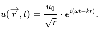
At large distances from the axis — that is, when  the wave field takes the form
 |
(1.2) |
 , the flux of the function
 remains constant;
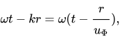
 the phase
  where
where  is the phase velocity of the plane wave.
Suppose that one system of coordinate
surfaces is formed by a family of
cylinders whose generators are
parallel to the z axis. Unless
specifically stated otherwise, these
cylindrical surfaces are not
assumed to be necessarily circular or
even closed. With respect to
each surface of the family,
the unit vectors ij, i£, i—
are arranged as shown in Fig. 64.
Thus, the vector ij is normal to the cylinder, ig is tangent to it and directed
along its generators, while ig is tangent to its surface and perpendicular
to ij and ig. Position with respect to the coordinate axes defined by these
three unit vectors is characterized by the coordinates u^, a^, z, and the
infinitesimal element of length equals
O Y
Fig. 64. Mutual arrangement of the unit
vectors on a cylindrical surface.
The generators are parallel to the z axis.
ds = i^h^du^ + ig V"" + h^2-
(1)
Let us now determine the components of the electromagnetic field associated with
the Hertz vector Π, directed along the z axis, so that Π1 = Π2 = 0,
in this chapter we will consider the medium not only isotropic and homogeneous
but also unbounded. Then, by (63) and (64), p. 40, the electric and
magnetic field vectors are given by the expressions
E(1) = rot rot Π, H(1) = ('s-^4-°) rot Π; (2)
since Π1 and Πg are equal to zero, then by (81) and (85), pp. 54—55, one can easily find
the components E^1) and H^1):
T^^) — J ^Σ^ p(2)_ 1 dt, ]
^^ ~" h1 dzdu^ ' '^ ~ h2 dzdu^ ' I
^^ ~ h1h2ldu^\h1 du\)~^ du^\kr dφ)\' J
Thus we obtained from the scalar function Π1 = ^
an electromagnetic field characterized by the absence of an axial or longitudinal
component of the magnetic vector. In view of the fact that Π is the electric
polarization potential, this field • can be called a field of electric
type (p. 39), but at the present time the term transverse magnetic field,
recently proposed by Schelkunoff ^), seems more appropriate.
Since Π1 is the rectangular component, it must
satisfy the scalar wave equation
or by (82), p. 54:
Elementary harmonic solutions of this equation have the form
(7)
where /(u1, u2) is a solution of the equation
(8)
In exactly the same way one can derive the particular form of the field from the second
Hertz vector Π*
E(2) = —rot Π*, H(2) = rot rot Π*; (9)
if Π* is directed along the z axis, then the components of these vectors are equal to
p(1) ' ^ p'(1)' ''^^^ py^i n f^n\
1 d'^Π! ,,, 1 d^Π!
(11)
"^ ~ h1h2ld^Kh1 du>^"^~^ da^^h2 dΦ^' .
The scalar function Π* is a solution of equation (5), and the field obtained from
«its field of magnetic type, or «transverse electric field:»
is characterized by the absence of a longitudinal component of E.
The electromagnetic field obtained by superposing the particular field types
obtained from Π and Π*, is general enough that it can
satisfy given boundary conditions on any cylindrical surface
with generators parallel to the z axis, i.e. on any coordinate
surface u1 = const, or u2 = const, or on the plane z = const. However, the choice
of these families of orthogonal surfaces is in practice limited to those
coordinate systems in which the variables in equation (8) separate.
6.2. Scalar and vector potentials. The transverse electric
and magnetic fields, defined in the previous section, possess
interesting properties which become apparent when considering the scalar
and vector potentials. Let us first consider the transverse magnetic
field, in which H^z = 0;
E(1) = —grad© — ^, B(1) = rot A,
φ = —divΠ, A = μ(ε—^+σ)Π.
In this case Π = Π1, whence
0:
dz *
dΦ
A = μ''—Π'°'^y A1 = A2 = 0.
(12)
(13)
(14)
The components E(1) therefore have the form
E1 ==
1 aφ
^?
d^Φ d^Φ
E
(1)
3 ' ' "
μσ
dt '
1
dφ
and the components B(1)
B"'=i
dA
du
,2 »
B?^.
r dA
h1 du^
B'=0,
(15)
(16)
where instead of A1 we write A without the index.
Note that in the plane z = const, the vector E(1) is irrotational;
consequently, in this transverse plane the line integral of E(1) between
any two points a and b does not depend on the connecting
path. Indeed, the element of length
in the plane z = const, has the form
ds = i1h1du1 + i2h2du2
and, consequently,
J
E(1)ds =
= -/(''"' + t''"'') = ^^"^-?(*^- ('^)
/.'
Fig. 65. Curve ab
depicts the cross-section of a
cylindrical surface
by the plane xy, in which
the vectors n and B(1) also lie
The potential difference or voltage
between any two points of the transverse
plane has a definite value at every moment, independent of
frequency or the type of cylindrical coordinates.
Further, one can note that the scalar function A plays the role of a stream
function for the vector B(1). Let the curve joining points a and b in Fig. 65,
represent the trace of a cylindrical surface intersecting the
plane z = const. Let us calculate the flux of the vector B(1) through a ribbon-shaped element of
the surface, bounded by the curve ab and having a width equal to unity
in the direction of the z axis. If n is the unit vector normal to this
surface, and ig is the unit vector directed along the z axis, then
(B^n) da = B(1) [n, ds] = i2 [ds, B(1)], (18)
where ds denotes the element of length along the curve. Expanding (18), we obtain
B^1)n da = h1B1du1 — h2B2du2 = — dA, (19)
whence
b
'J B^1)n da = A(a) — A(b). (20)
a
The magnetic flux through any strip of unit width on a
cylindrical surface, passing through two points in the plane z = const.,
does not depend on the shape of the strip.
If we express the components E^1) and B^1) through the scalar function Ψ,
it is then easy to show that
ΦB^1) — E'A' = 0, (21)
and, consequently, the projection of the vector E^1) onto the plane z = const, is everywhere
perpendicular to the vector B^1). In the transverse plane the family of curves
φ = const, (equipotential lines) and A = const, (lines of «flow»
of the vector B^1)) coincide. From (14) and (7) it is clear that for harmonic variation
in time the equipotential lines are
f(u1, u2) = const., (22)
where f(u1, u2) satisfies equation (8).
The transverse electric field "possesses similar properties, only the
roles of the electric and magnetic vectors are interchanged. According to (35), p. 37:
D(2) = —rot A*, H(2) = »—gradφ*——- —μA* (23)
φ*=_divΠ*, A*==Π'εμ« (24)
Setting Ψ = Π2, Π1==Π2 = 0,* we obtain
dΠ .* dΦ .* .* _.
φ*==—•|j, Az=Π-εμ, A1 = A2 = 0; (25)
The components of the field vectors will therefore be:
1 aA* ^(2) 1 dA*
(27)
The projection of H(2) onto the transverse plane is irrotational, and
consequently, the curvilinear integral representing the magnetomotive force
between two points in this plane is independent of the path of integration:
'J H(2)ds = φ* (a) — φ* (b). (28)
In a similar way, the flux of the vector D(2) through a strip of unit width,,
shown in Fig. 65, depends only on the endpoints
b b
'J D(2)n da = 'J dA* = A*(b) —A*(a). (29)
a a
The projection of H(2) onto the plane z: = const, is everywhere perpendicular to the vector D(2).
It follows that the families of curves φ* = const, and A* = const, coincide.
The field D(2), H(2) is in this sense conjugate to the field E(2), B(2).
6.3. Impedances of harmonic cylindrical fields. Let us assume,,
that time enters only through the harmonic multiplier e-iωt. Then the potentials,
and the components of the field strengths of the transverse magnetic field have the form
φ = -p ih', A = — i (μεω + iμσ) ^^ (30)
Z(1)=__iω i', Z(1)-^=.i' H(1)=0, '(32)
where h2 = μεω+iμσω. The upper sign refers to waves propagating
in the positive direction along the z axis, the lower — to waves
propagating in the negative direction.
The set of impedances relating to the field strengths can
now be determined on the basis of section 5.6. The value of the impedance depends,,
of course, on the direction in which it is measured. By definition
According to p. 252, the intrinsic impedance of a homogeneous isotropic medium;
for plane waves is
Ζ0 = i'
—b-=^^ (34).
so that (33) can be represented as
Z(1) = ±Ζ0- (35)
Similarly, the impedances in the directions of the transverse axes can be
determined by the relations
Z(1) = -Z^h, E?,==Z^h''. (36)
The sign of the components of the electric and magnetic vectors is determined,,
of course, by the positive direction of the Poynting vector. Since H(1)
is equal to zero, the current component represented by the terms E(1) and I(1)
is absent, and the corresponding impedances are infinite. Substituting
the corresponding expressions for the field components into (36), we obtain
The determination of the corresponding impedances for the harmonic components
of the transverse electric field needs no further explanation.
The potentials and field vectors in this case have the form
φ* = zp Πi, A* = — iμεω'i', (38)
Z(2)' = '>"^^. Z'—^^Ξ' H(2)' = «. (39)
Z' = ±Ζ0— "Z' = ±i (h2—k2)^^. (40)
From these relations the impedances are computed:
Z(2) ik dΦ Z(2) ik du^ (43)
This gives rise to a curious series of relations
Z(1)Z(1) _ Z(2) _ Z(1)Z(2) _ Z(2); • (44)
WAVE FUNCTIONS OF THE CIRCULAR CYLINDER
6.4. Elementary waves. The simplest case of separable variables
;is the one in which the family u2 == const, represents
a set of coaxial circular cylinders. Then, according to 1, p. 56,
u1 = r, u2 = θ, h1=1, h2 = r, (1)
and equation (8) of section 6.1 takes the form
where the variables are easily separated if we represent f(r, θ) as a
product
f=f1(r)f2(θ), (3)
in which f1(r) and f2(θ) are arbitrary solutions of the ordinary differential
equations
'#+p'%= 0. (5)
The parameter p, just like h, is a separation constant; its choice
is dictated by the physical requirement that the field be single-valued at a fixed
point in space. If inhomogeneities and discontinuities of the medium are
excluded, as is assumed in the present chapter, then the field must ,
be periodic in θ and the values of p are restricted to integers n = 0,
±1, ±2, ... On the other hand, if the field is represented by particular
solutions of equations (4) and (5) in a sector of space bounded by
the planes θ = θ1 and θ=θ2, then the parameter p must in general take
Equation (4), which the radial function f1(r) satisfies, is
Bessel's equation. Its solutions could be called Bessel
functions, but since this name is usually applied only to that
particular solution Jp (√k2 — h2 r), which is finite at the axis r = 0, we
will call the arbitrary particular solution of equation (4) a circular
cylindrical function and will denote it by f1 = Zp(√k2—h2 r).
The argument of the function is √k2—h2 r, and p is called its order. Thus
the particular solutions of the wave equation (5), p. 310, periodic in φ and θ,
can be constructed from elementary waves of the form
The propagation constant h, in general, is complex: consequently,
the field is not necessarily periodic along the z axis. An explicit expression for h
as a function of the frequency ω and the constants of the medium can be obtained only by specifying
the behavior of Ψ on the cylindrical surface r = const, or in the plane z = const.
6.5. Properties of the functions Zp(ρ). Assuming the reader is familiar with
the theory of Bessel's equation, it is nevertheless useful to give, for reference, a review of the most important
properties of the solutions of this equation.
If in equation (4) we replace the independent variable with ρ = √k2—h2r,
then we find that Zp(ρ) satisfies the equation
which is characterized by a regular singularity at ρ = 0 and
an essential singularity at ρ=∞. The Bessel function Jp(ρ) or the
cylindrical function of the first kind is the particular solution of (7), finite at
ρ = 0. It can thus be expanded in a series of increasing
powers of ρ, and since in the plane of the complex variable ρ there are no other
singularities besides the points ρ = 0 and ρ = ∞, this series obviously converges
for all finite values of the argument. For any p, real or
complex, and for real or complex ρ, the expansion holds
the expansion
∞
If in (7) we replace p with —p, the equation remains unchanged;
consequently, for non-integer p the second fundamental solution can be obtained
from (8) by replacing p with —p. But if p==n is an integer, then Jp(ρ)
becomes a single-valued function of the point. The gamma function Γ(n+m+1)
is replaced by the factorial (n+m)!, so that
J'n(ρ)==Σm,\m;^)|(') (n = 0,1,2....). (9)
The function J-n(ρ) obtained thus is not independent of (9), but is related to it
by the relation
J-n(ρ) = (-1)"Jn(ρ). (10)
so that to find the second solution one must resort to some
other known method.
The Bessel function of the second kind is defined by the relation
This solution of equation (7) is independent of Jp(ρ) for all
values of p, but the right-hand side takes the indeterminate form 0/0 for integer p.
However, its value can be computed in the usual way, by differentiating
the numerator and denominator with respect to p and then taking the limit as p→n.
The resulting expansion is rather complicated ^); we shall give only the first term,,
valid in the vicinity of the origin:
N0(ρ)=^-^ln|, Nn(ρ)≈ ~^'^' (1)" (n=1.2.---), (12)
where γ=1.78107 and |ρ| << t. A characteristic property of functions of the second kind
is the presence of a singularity at the origin. Because they
become infinite at ρ = 0, they cannot be used to
represent fields which, by their physical meaning, are finite
in the vicinity of ρ = 0.
Further information on the character of the functions Jp(ρ) and Np(ρ) is given by studying;
their behavior for very large values of ρ. The expansions in the vicinity of
the origin converge for all finite values of ρ; Jp(ρ) and Np(ρ)'
are everywhere analytic functions of p and ρ, except at the points ρ = 0 and.
ρ=∞. However for very large ρ the series converge so slowly'
that they become useless for practical calculations, and here
representations of these same functions are used instead, in the form of series in
inverse powers of ρ. Indeed, one can show that Bessel's equation
is formally satisfied by the expansions
Jp(ρ)= √(2/πρ) [Pp(ρ)cosσ—Qp(ρ)sinσ], (13)
Np(ρ)=√(2/πρ) [Pp(ρ)sinσ + Qp(ρ)cosσ], (14)>
Pp(ρ)— 1— (4p2—1)(4p2—9)' ,
2! (8ρ)2 '
Qp(ρ)—(4p2—1) + (4p2—1)(4p2—9)(4p2—25) , ' '
8ρ ' 3!(8ρ)3—: +•••' (16)
where the phase angle σ is given by the expression
σ=ρ-(p\+()l. (17)
It turns out, however, that these series diverge for all values of p and ρ,,
consequently, they do not have exactly the analytic properties of the functions^
which they are supposed to represent. On the other hand, for
large ρ the first terms rapidly decrease in magnitude, and in this sense
the series are «semi-convergent». It can be shown that if one breaks off the
expansion near the term where the subsequent terms begin to grow, or,
before that term, then the expansion gives an approximate value of the function,
and the resulting error can be estimated. The larger p is, the closer
the value of the sum of several first terms comes to the true value of the function.
For this reason such representations are called asymptotic.
Note that for sufficiently large ρ
Jp(ρ)≈√(2/πρ) cos(ρ-pπ/2—π/4) (18)
__ |ρ|>>1, |p|«'|ρ|.
Np(ρ)≈√(2/πρ)sin(ρ-pπ/2—π/4). (19)
At very large distances from the origin, cylindrical functions
of the first and second kind relate to each other as cosine and sine,
«and they attenuate with growth of ρ owing to the factor 1/√ρ". These functions are convenient
for representing standing cylindrical waves.
By analogy with exponential functions, one can construct a linear
combination of the solutions Jp(ρ) and Np(ρ), giving functions related to travelling'
waves. Bessel functions of the third kind, or, as they are more often
called, Hankel functions, are defined by the relations
Hp(1)(ρ) = Jp(ρ)+iNp(ρ) (20)
Hp(2)(ρ)=Jp(ρ) — iNp(ρ). (21)
From the preceding formulas it is easy to find that for very large ρ
Hp(1)(ρ)≈√(2/πρ)ei(ρ—pπ/2—π/4), (22)
(2).
|ρ|»1, |p|:>|ρ1
2p + π
/ / * "p -T^ \
Hp(2)(ρ)≈√(2/πρ)e-i(ρ—pπ/2—π/4). :(23)
To the expansions of the functions themselves in series we add for reference;
some of the most important recurrence formulas:
Zp-1 + Zp+1 = (2p/ρ)Zp, (24)
-— = -Zp-1-1Zp,, (25)
-'[ρpZp]=ρp Zp-1', (26?)
-'[ρ-pZp(ρ)]=-ρ-p Zp+1'. (27)
6.6. Field of circular cylindrical wave functions. Inside a
homogeneous isotropic region, any electromagnetic field can be represented
by a linear combination of elementary wave functions
Ψnih = einφJn(√k2—h2 r)e ± ihz-iωt, (28)
Ψnh = einφHn(1) (√k2—h2 r) e± ihz-iωt (29)
For finite regions including the axis r = 0, only the functions
(28) apply; at large distances from the source the functions
(29) must be used, since they asymptotically pass over, according to (22), into a radially
diverging wave. Each elementary wave is defined by the triple
of parameters n, h, k. When h = 0 the field is symmetric about the axis; when h≠0
propagation occurs only in the radial direction, and the field is
strictly two-dimensional. It can be said that functions of the form (28) and (29)
represent inhomogeneous plane waves. Planes of constant phase
propagate along the axis z with velocity V = ω/α, where α is the real
part of h, but the amplitudes in these planes are functions of r and θ. Such
waves can only be produced by sources located at finite
distances from the origin, or in media with discontinuities.
The plane waves studied in the preceding chapter are homogeneous in the strict sense
of the word, since planes of constant phase are also planes of
constant amplitude. They can exist only in infinite
homogeneous media with sources of excitation infinitely far away.
From the formulas derived in section 6.3, one can express the impedances and
the components of the field vectors in terms of the wave function Ψ:
Z(1) _
ωμ
— √h2
/k2
h2r
Z(1) _ _H mωh
Z z ' ' to •
/k2
(30)
Er — — ''^ ^ '
dρ
Z(1) _4_ ih dΦ
;(1)
Er = (k2
tB'z = 0.
/Z2L-, (31)
(32)
Similarly, for the transverse electric field
dZn(ρ)
ωμ
√h2-k2' Zn(ρ)
Hr' = ±iωh
k2 — h2 r '
Z(2) = ±;:. (33)
E'' = 0, ' (34?)
Hz' = (k2 —h2). (35)
If initial conditions are given on some plane or
cylindrical surface, then the solution is formed by superposition of elementary
wave functions. For fixed values of ω (or k) and h, the following
expressions are obtained for the resulting field in cylindrical coordinates:
Ez = ih
1
α.
dΦ.
∞
\
n
n z
— Σnbn'Ψn^
n-
-∞
dω
n = —∞
∞
n
n = —∞
Σ
n= ~<∞>
∞
n3 1
\m
n = —∞
(36?)
« = — ∞ μ = — ∞
∞ ∞
dr
Hz=
n — —∞
n= —∞
∞
Hz={k2~h2) Σ k'Ψn,
n = —∞
(37?)
where an and bn—are coefficients
determined from the initial conditions.
The direction of propagation is positive or negative depending on the sign of h.
INTEGRAL REPRESENTATIONS OF WAVE FUNCTIONS
6.7. Construction from plane waves. If ζ measures the distance along
an arbitrary axis, whose direction with respect to a fixed
frame of reference (x, y, z) is defined by the unit vector n, then, according to
sections 5.1—5.6, the simplest type of plane wave can be represented by the
function
in which the constants k and ω can be either
real or complex. Let
R—be the radius vector drawn from the origin to the observation
point, whose rectangular coordinates
are x, y, z. Then the phase of the wave function
at a given moment of time is measured by the quantity
ζ = nR=n1x+n2y+n3z. (2)
The direction cosines nx, ny, nz of the vector n
are more conveniently expressed through the polar angles α and β,
shown in Fig. 66:
nx = sin α cos β, ny = sin α sin β, nz = cos α, (3)
Fig. 66. The phase of an elementary;
plane wave is measured
along the axis ζ, whose direction
is determined by
the unit vector n. The observation
point has the radius
vector R.
whence
Ψ = ei(k(x sin α cos β+y sin α sin β+z cos α)-iωt) (4")
By varying the parameters α and β, one can give the axis of
propagation any direction. Each direction of propagation is associated with an amplitude
g(α, β), depending only on the angles α and β. Since the field equations in the
case under consideration are linear, the solution can be constructed by
superposition of plane waves of the same frequency, but with different directions
of propagation and with corresponding amplitudes ^):
Ψ(x,y, z, t) = e-iωt 'J dα 'J dβg(α, β) ei k(x sin α cos β+y sin α sin β+z cos α) E'
If the angles are real, then α varies from 0 to π, and β from
0 to 2π. Such a solution, from a mathematical point of view, is by no means
the most general, since (5) satisfies the wave equation both for
real and for complex values of the parameters α and β, and
we shall soon find that complex angles must indeed be
included in the consideration if we wish to represent by such an integral
any field whatsoever.
For real ω the wave function defined by equation (5),
is harmonic in time. To represent a field which on a
given coordinate surface varies with time in a more
complex manner, it is necessary to sum or integrate (5) over the
parameter ω. Let us define the vector propagation constant as
k = ωn, whose rectangular components are equal to ,
k1 = k sin α cos β, k2 = k sin α sin β, k3 = k cos α.
(6).
so that the elementary plane wave function can be written in the form
Ψ=eikR-iωt (7)
Substituting (7) into the wave equation
we find that the components of k must satisfy a single
relation
k12+ k22+ k32=ω2(μεω2 + iμσω) = k2, (9)
and are otherwise completely arbitrary. Thus, of the parameters k1,
k2, k3, ω one can choose arbitrarily any three parameters, after which
the fourth is determined by equation (9). ^^
Suppose that on the plane z = 0 the function Ψ is given:
Ψ(x,y, 0,t)=f(x,y;t).
The desired solution will be
Ψ(x, y, z, t) =
∞ ∞ ∞
—∞ —∞ —∞
Σ
where k1, k2 and ω—are real variables, and k3 — is a complex quantity,
determined by the relation
k3=√μεω2+iμσω—k1—k2i. (11)
The amplitude function g(k1, k2, ω) is such that
∞ ∞ ∞ *
f(x,y,t) = (2π)3 'J 'J 'J g(k1,k2,ω)ei(k1x+k2y-ωt)dk1dk2dω. (12)
— ∞ —∞ -∞
If f(x, y, t) and its first derivatives are piecewise continuous and absolutely
integrable, then g(k1, k2, ω) is the Fourier representation of the function
f(x,y, t) and equals
∞ ∞ ∞
3
g(k1, k2, ω) = (2π) 'J 'J 'J f(x, y, t)e-i(k1x+k2y-ωt) dx dy dt (13)
—∞ —∞ —∞
At z = 0 each harmonic component propagates along the z axis
with velocity v = ω/k3, but since k3=√ω2(με — k12 — k22) is not a
linear combination of ω, k1 and k2, the initial disturbance f(x, y, 0), obviously,
will not propagate without distortion of form, even in the absence of a dissi-
pative term. More precisely, no general solution of equation (8) of the form
Ψ(x,y,z,t) exists.1
Equally well one could specify the function Ψ(x, y, z, t) throughout
all of space at the initial moment of time t=0. Let, for example,
Ψ(x,y, z, 0) = f(x, y, z). The field is represented as a triple integral
∞ ∞ ∞
—∞ —∞ —∞
in which k1, k2, k3—are real variables, and ω—is a complex'
quantity, determined from (9):
ω=±√a2(k12+k22+k32)—b2, (15)
where a==1/√με, b =σ/2ε (see p. 264). The amplitude or weighting function
g(k1, k2, k3) is such that
∞ ∞ ∞-
f(x, y, z) = (2π)3 'J 'J 'J g(k1, k2, k3) ei(k1x+k2y+k3z) dk1 dk2 dk3. (16)
-∞ —∞ —∞
If f(x, y, z) possesses the necessary analytic properties,
then its Fourier representation exists and has the form
∞ ∞ ∞
3
g(k1,k2,k3)==(2π)-3 'J 'J 'J f(x,y,z)e-i(k1x+k2y+k3z)dxdydz. (17)
-∞ —∞ ——∞
In the preceding sections we considered only positive or
diverging waves, and the initial conditions were imposed only on the
function Ψ itself. If certain conditions are imposed both on the function Ψ and
on its derivative with respect to one of the four arguments, it is necessary
to include in the consideration both positive and negative waves, in
accordance with the methods described for the one-dimensional case in sections
5.8, 5.9 and 5.10.
6.8. Integral representations of the functions Zn(ρ). In an arbitrary
system of cylindrical coordinates u1, u2, z, the wave equation (6),
p. 310, is satisfied by the function
Ψ = f(u1, u2)]eihz-iωt, (18)
where h and ω—are real or complex constants. In the notation of
the preceding paragraph h =k3 = k cos α, and since k = √μεω2+iμσω, the
angle α, formed by the direction of the plane-wave components with the z axis,
is likewise constant. In other words, the elementary cylindrical wave (18)
can be decomposed into homogeneous plane waves whose directions
form a circular cone about the z axis, but the half-angle of the cone
is in general complex:
f(u1, u2) = 'J g(β) eik sin α (x cos β+y sin β) dβ, (19)
where x and y should be expressed in terms of the cylindrical coordinates u1 and u2.
In the coordinate system of the circular cylinder we have x=,rcosθ,
y = rsinθ, whence .,. ,
xcos β+ y sin β=rcos(θ—β).
In the notation of the preceding paragraph we obtain further
krsinα=r√k2—h2=ρ, (21)
so that
f(r, θ) = 'J g(β)eir√k2—h2 cos (θ-β) dβ. (22)
Let us now replace in (22) the variable of integration β by σ = β — θ ^
we note that since the variables in the equation for f(r, θ) separate, then
g(σ+θ) can be represented as a product of two functions, each of
which depends only on one variable:
g(β)=g(σ+θ)=g1(σ)g2(θ); (23)
consequently,
f(r, θ)=f1(r)f2(θ) = g2(θ) 'J g1(σ) eiσ+θ dσ. (24)
The angular function g2(θ) must, evidently, be some linear
combination of the exponential functions eiθ and e-iθ, and the amplitude or weighting
factor g1(σ), must be chosen so that the radial function f1(r)
satisfies equation (4), p. 314, which in terms of the argument ρ has the form
Substitute into (25) the integral
* f1(ρ) = 'J g1(σ)eiρsinσdσ. (26)
Differentiating under the integral sign, we obtain
d/dρ = 'J i cos σ g1(σ) eiρsinσ dσ, d2/dρ2 = — 'J cos2σ g1(σ) eiρsinσ dσ. (27)
consequently, according to (25),
'J (ρ2 sin2θ + iρcosθ—n2) g1(σ) eiρsinσ dσ = 0. (28)
We shall further transform this equation by integration by parts.
Equation (28), evidently, is equivalent to the following:
'J [g1(σ) d/dσ2 — n2 g1(σ) eiρsinσ] dσ == 0. (29)
If P and Q are two functions of σ, then
which when applied to (29) gives
The first of these two integrals can be reduced to zero if
one chooses the contour of integration such that the expression under the sign of
the derivative has the same value at the initial and final points; the second
integral vanishes if the integrand is equal to zero.
Consequently, (26) is a solution of Bessel's equation if g1(σ) sat-
isfies the equation
'g1''+ p2g1-0, ' ' : (32)
and the path of integration is such that
Equation (32), evidently, is satisfied by the function eipσ. However, as we
shall see, in order that f1(ρ) be identical with the cylindrical
function Zp(ρ), defined in section 6.5, one must add a constant factor
—e-iπp/2. Thus, setting
. (34)
we obtain the Sommerfeld integral representation of the cylindrical
functions 1):
' Zp (ρ) = 1/(2πi) 'J ei(ρ sin σ+pσ) dσ, (35)
c
where the contour C is such that
(ρ sin σ ~ p) ei(ρ cos σ+pσ) | = 0. (36)
The distinction between the various particular solutions Jp(ρ), Np(ρ), Hp(ρ)
is now reduced to the difference in the contours of integration in the plane of the complex
variable σ. Let us first consider the simplest case, when
p = n is an integer. Then it is evident that if the integration
is performed along the real axis of σ from —π to +π or over any
other interval of length 2π, then condition (36) is satisfied, and the definite
integral
Jn (ρ) = 1/(2π) 'J ei(ρ sin σ-nσ) dσ (37)
is a solution of Bessel's equation. That the function defined
by equation (37) is indeed identical with the particular solution (9), p. 315,^
can be verified by expanding eiρcosσ in a series in the vicinity of the point ρ = 0 and inte-^
grating this series term by term.
In the general case, when p is not an integer, or in order to
obtain another independent solution, for (36) to vanish
at the endpoints, the variable σ must be assigned complex values..
Let σ = γ+iη. Then
ip cosσ + ipσ = p(sin γ sh η) — pη + i(p cos γ ch η + ipγ) (38)
If p is complex, we set p = a+ib, where a—is an essentially posi-
tive quantity. Then by a suitable
choice of γ and η, one can make
the real part of (38) an infinitely large negative
quantity, while at
this exp(ip cos σ + ipσ) → 0. This condition is satisfied, for example, if one sets
η→+∞, and for γ take the values —π/2 or +3π/2; but this
exponential function also vanishes as η → —∞, provided only that
γ = +π/2. In order that (35) represent a solution of Bessel's equation,
it is only necessary that the contour C join any two of these points.
Sommerfeld chose as a pair of fundamental solutions two
integrals
Hp(1)(ρ)=
•ipσ
'J
eip cos σ+ipσ dσ
(39)
—+∞
cos σ + iβσ
dσ.
(40)
-γ—∞
The contour C1, along which the integral (39) is taken, begins at η = ∞, γ = —π/2,
crosses the real and imaginary axes at σ = 0 and ends at
η=—∞, γ=+π/2. The contour C2, along
which the integral (40) is taken,
begins at the endpoint of contour C1,
crosses the real axis at
σ = π and ends at η = ∞,
γ = 3π/2. Both contours are shown in
Fig. 67. The point of intersection with the
real axis is, of course, immaterial
for the determination of the function. The contours
can be deformed arbitrarily,
provided only that they
begin at the infinitely distant
central point of one shaded
region and end at the
corresponding point of the other
shaded region.
The advantages of routing C1 and
C2 through the points γ = 0 and γ = π
of the real axis become evident
when computing the integrals (39) and (40)
for very large values of ρ. If the real part of ρ is very large,
then the factor exp(ip cos σ) becomes vanishingly small at all points
of the shaded regions in Fig. 67, except in the immediate vicinity of the points
η = 0, γ = 0, —π, — 2π, ... At these points the real part of ip cos σ,
according to (38), equals zero, however large ρ may be; consequently, if
C1 and C2 are drawn as shown in Fig. 67, then the total value of the contour
integral is determined by the value of the integral taken only in the vicinity of
the origin
and the point η=0, γ = π. Out of the shaded region, in
which the values of the integrand are vanishingly small, the contour C1 passes
through a steep «pass» or «saddle point», where the integrand
is large, and then moves onto another shaded plane,
where the function decreases sharply, and the value of the integral over this region again
becomes negligibly small. The contour C2 has a similar saddle point
at η = 0, γ = π.
To reduce the integration to as short as pos-
sible section of the contour, one must approach the pass along the line of steepest
ascent, and descend from the «summit» into the «valley:» along the line with
the steepest descent. In this case this means that the contours C1 and C2.
must cross the axis at an angle of 45°* Debye *) used the behavior of the
integrals (39) and (40) in the vicinity of the saddle points to compute,
asymptotic expansions of the functions Jp(ρ) and Hp(1)(ρ). For ρ, very
large compared with unity and with the order p, one obtains relations
(22) and (23), p. 317, which shows the identity of the integrals (39) and (40)
with the Hankel functions defined in section 6.5. Debye also considered
the case where p is greater than the argument ρ; his results were
improved and extended by later investigations.
The representation of Jp(ρ) for non-integer p as a contour integral
follows directly from the relation
Jp(ρ)=1/2[Hp(1)(ρ)+Hp(2)(ρ)], (41)
whence
π
Jp (ρ) = 1/2π 'J eip sinσ+iσp dσ. (42)
α
3
The contour C3, shown in Fig. 67, represents an admissible
deformation of the contour C1+C2.
6.9. Fourier—Bessel integrals. We have shown how, from a
scalar function Ψ in cylindrical coordinates, two basic types of
electromagnetic field are derived. If the cylindrical coordinates are circular,
then Ψ is obtained, in general, by superposition of elementary waves of the type
of the particular solutions (28) and (29), p. 317. Our task now is
the following: given the values of Ψ(r, θ, z, t) at the moment t=0 in the plane z=0'^
it is required to find Ψ for all other values of z and t.
Suppose that at t = z = 0 the function Ψ=f(r, θ). We shall assume.
f(r, θ) is a bounded and single-valued function of the variables, piecewise
continuous together with its first derivatives. Then f(r, θ) must be
periodic in θ and can be expanded in a Fourier series, whose coefficients,
are functions of r alone:
2π
f(r,θ)=Σfn(r)einθ, fn(r)==±'Jf(r,θ)e-inθdθ. (43)
n = —-∞
If f(r, θ) tends to zero as r→∞ so that convergence is ensured
∞
of the integrals 'J|fn(r)|2rdr, then each coefficient fn(r) can be.
0
represented by a modified Fourier integral 2).
Let us consider a function f(x,y) of two variables, admitting the
Fourier integral representation
~∞ —∞
*) Debye, Math. Ann. 67, 535, 1909, see also Watson, loc. cit., p.
Let us now perform a transformation to polar coordinates both in the coordi.-
nate space, and in the k-space:
x r=rcosθ, y = r sin θ,
k1 = kcosβ, k2=k sinβ,
so that in the notation of the preceding paragraphs >. λ=k sin α = √k2— h2.
Then k1x+k2y=krcos(β—θ), and (44) as a volume integral in k-
space takes the form:
2π
f(r, θ) = 1/(2π) 'J k dk 'J dβ g(k, β) eikrcos(β—θ). (46)
0 0
It is easy to disclose the physical meaning of this representation. The function
exp[ikr cos(β — θ) — iωt] represents a plane wave with propagation
constant k, travelling in a direction perpendicular to the z axis and
making an angle β with the x axis. Each plane wave is multiplied by the
amplitude factor g(k, β); then the waves are summed first over β
from 0 to 2π, and then over the propagation constant or spatial
frequency k.
The Fourier representation of the function f(x,y) has the form
∞ ∞
g(k1, k2) = 1/(2π)2 'J 'J f(ξ, η) e-i(k1ξ+k2η) dξdη, (47)
—∞ —∞
which, on going over to polar coordinates ξ = ρ cos μ, η = ρ sin μ. gives
∞ 2π •
g(k, β) = 1/(2π)2 'J ρdρ 'J dμf(ρ, μ) e-iρk cos(μ-β). (48)
0 0 •
Finally, suppose that f(r,θ)=fn(r)einθ. Then
∞ ' 2π
g(k, β) = 1/(2π)2 'J ρdρfn(ρ) 'J e-iρk cos(μ-β)+inμdμ (49)
0 0
which after change of variable σ = μ — β — π gives
gn(β) = in(—1)n 'J fn(ρ) Jn(kρ)ρdρ=gn(k)einβ, (50)
0
Similarly (46) takes the form:
∞ 2π ( 3 )
f(r, θ)=fn(r)einθ=1/(2π) 'J k dk gn(k) 'J e ikrcos(β-θ)+in(θ+β) dβ (51)
0 0,
or, if we set σ=β — θ:
∞
fn(r)einθ=einθ 'J gn(k) Jn(kr) k dk, (52)
Thus we obtain a pair of Fourier—Bessel representations:
∞
fn(r) = 'J gn(k) Jn(kr) k dk, (53)
0
∞
gn(k) = 'J fn(ρ) Jn(kρ) ρ dρ. (54)
0
The function
∞
∞ _
Ψ=e-iωt Σ einθ'J gn(k)Jn(kr)e±ihz-iωt2πk dk (55)
n=—∞
is a solution of the wave equation in circular cylindrical
coordinates, which at t = 0 reduces to f(r, θ) on the plane z ~ 0. But this,
obviously, is not the most general solution satisfying these conditions, since
we still have at our disposal two more parameters ω and h, on which
only one condition h2 = μεω2+iσμω is imposed. For real ω
one can, by superposition of harmonic wave functions of type (55),
represent an arbitrary law of variation of Ψ with time in the plane z = 0. If
we consider both positive and negative waves, one can specify at z=0 the values of both
Ψ and its derivative. Consideration of such problems
was given in chapter V.
6.10. Representation of a plane wave. The Fourier—Bessel theorem gives a very
simple way of representing an elementary plane wave through
cylindrical wave functions. Let a wave with propagation constant k
travel in a direction defined by the unit vector n, whose spherical
polar angles relative to a fixed frame of reference equal
α and β, as shown in Fig. 66, p. 319. Then
Ψ = eik sin α (x cos β+y sin β) · eikz cos α-iωt (56)
and our task reduces to representing the function
f(x, y) = ei(kx sin α cos β+ky sin α sin β) = eikr sin α cos(β—θ) (57)
in the form of a series
∞
f(r,θ)= Σ fn(r)einθ, (58)
n=—∞
According to (43), we have
2π
fn(r) = 1/(2π) 'J eikr sin α cos(β-θ)-inβ dβ, (59)
0
Replacing β — θ with σ, this becomes
fn(r) = ein(α+π/2) Jn(kr sin α), (60)
and we obtain a useful expansion
∞
eikr cos(β-θ)= Σ in Jn(kr sin α)ein(β-θ). (61)
Certain other well-known series are direct consequences
of this expansion. Thus, if we set ρ = kr sin α, and θ—β=φ—π/2,
relation (61) takes the form
∞
eiρ sinφ= Σ Jn(ρ)einφ (62)
n=—∞
which, after separation into real and imaginary parts, gives
∞
cos(ρ sin φ)= Σ Jn(ρ)cos nφ,
n = —∞
∞ I
• sin(ρ sin φ)= Σ Jn(ρ)sin nφ' j
n= —∞ J
ADDITION THEOREM FOR CIRCULAR CYLINDRICAL WAVES
' 6.11. From the formulas of the preceding section one can derive a series of important
relations, relating to the translation of the propagation axis parallel to itself.
In Fig. 68, O and O1 denote
the origins of two rectangular systems
of reference. The plane of the drawing coincides
'^/ '' \~ ^ with the xy plane of both systems, and the axes x1'
-^~ —^ ^^^ passing through O1, are parallel
'' ' ' ' to the corresponding axes x, y, z. The function
Jn(λr1)einθ1, multiplied by exp(±ih z1—iωt)^^
O ' "' represents an elementary cylindrical
Fig. 68. Translation of the frame of reference. wave, referred to the axis z1. We want to
express this cylindrical wave in the form of a
sum of cylindrical wave functions, referred to the parallel axis
z, passing through O.
Let us first write
1 r >''1 cos σ + i(u + θ1)
—π
From the drawing it is clear that θ1 = θ + 'π'
r1 cos θ1 = r1 cos(ψ — θ) = r — r0 cos(ψ — θ0),
r1 sin θ1 =
r1cos(ψ — θ) = r—r0cos(ψ — θ0), I
r1 sin(ψ — θ) = r0 sin(ψ — θ0). J
(3)
Moreover, because of the periodicity of the integrand, (1)
is equivalent to
From (2) it follows that
r1 cos(θ — ψ) = r cos θ — r0 cos(θ +θ — θ0), (4)»
whence
1 J[r cosθ—r0 cos(ψ+θ—θ0)+r0](φ+θ—π/2)
According to (61), p. 327,
' ^^.'^'^ • ∞
πk
By virtue of uniform convergence one can change the order of summation,
and integration:
— π
∞
m =—∞
∞
When θ1 is replaced by θ+'ψ' this expression takes the form
∞
m = —∞
A similar expansion for the wave function H1(1)(λr1)e iθ1 can be obtained-
from the integral
Hn(1)(λr1).einθ1 = i'J e iλr cosσ-inσ+iσ(θ- θ) dσ,
(9)
where C1 — is the contour shown in Fig. 67, p. 324, shifted by a value
along the real axis, ensuring the vanishing of the exponential
function at the endpoints. Replacing the exponent by (2), we find that
When |r| > |r0 cos(ψ — θ0)| one can, proceeding entirely analogously,
arrive at the expression
When r0==0 both centers coincide; Jm(ρ) = 0 for all values of m, except-
zero, and J0(0) = 1• the value is zero, and the right and left sides of equation (11),,
are obviously identical. The validity of the expansion can also be verified
for very large r and r1, since in this case the Hankel functions
can be replaced by their asymptotic representation (22), p. 317. The angle θ-
is approximately zero, and r1≈r — r0cos(θ — θ0). The amplitude
factor "√2/πr1 can without appreciable error be replaced by √2/πr, but the term,-
r0cos(θ — θ0) in the phase should be retained. Then (11) takes the form
m = —∞
and the right-hand side of (12) in turn is, according to (61), p. 327,,
the exact expansion of the plane wave standing on the left-hand side. Indeed,
as r0 increases without bound, the diverging cylindrical wave
function, defined by (11), must asymptotically transform into a plane
wave.
When |r|<|r0cos(θ — θ0)| the expansion (11) does not converge and is replaced,
by the expansion
Jn(λr)einθ= Σ Hn+m(1)(λr0)Jn+m(λr)eimθ0, (13).
which is finite at r = 0. At this point Jn+m(λr) equals zero, except for
m = — n. Moreover; θ = π + θ0 — π «» since Hn(1)(ρ) = einπHn(2)(ρ),, then,
evidently, the right and left sides of equation (13) are identical. In the other
limiting case of very large r0 we set r1==r0 — r cos(θ—θ0)
and with the help of the asymptotic representations of the Hankel functions we find that
(13) tends to
m — —∞
i.e. to a plane wave propagating from O1 to O along the line
joining these two centers.
WAVE FUNCTIONS OF THE ELLIPTIC CYLINDER
6.12. Elementary waves. Circular cylindrical functions are,
essentially, a degenerate form of elliptic wave functions,
obtained by setting the eccentricity of the cylinders equal to zero. In
elliptic coordinates the study of the field and the properties of the functions must inevitably
prove more complex than in circular coordinates, but on the other hand the results
are considerably more interesting.
According to 3, p. 57, we set
u1=ξ, u2 = η,- ξ>1, —1<η<1, (1)
'h1 = c0√|ξ2—η2|/(ξ2-1) . h2 = c0√|ξ2—η2|/(1-η2). (2)
Substituting this into (8), p. 310, we find that f(ξ, η) must satisfy
the equation
—+c02(k2—h2)(ξ2—η2)f=0. (3)
This equation in turn is easily separated if we set f=f1(ξ)f2(η)'
which gives:
d/dξ[(ξ2-1)df1/dξ]+[b-c02(k2—h2)ξ2]f1 = 0, (5)
where b is an arbitrary separation constant. Thus, f1(ξ) and f2(η)
satisfy one and the same differential equation.
Equations (4) and (5) are special cases of the corresponding
Mathieu equation 1)
(1—z2)'w" — '2(a+1)zw'+(b~c2z2)w=0, (6)
which are obtained if one sets the parameter a = ½. These equations
are characterized by an irregular singularity at infinity and regular
singularities at z=±1. As ξ→∞ (4) reduces to Bessel's equation.
A significant simplification of (4) and (5) can be achieved by a change
of the independent variables. Let
ξ = ch u, 'η = cos v, (7)
1) E. T. Whittaker and G. N. Watson, loc. cit., chapters X and XIX; I n
so that the transformation to rectangular coordinates is expressed by
the equations'
x = c0 ch u cos v, y =c0 sh u sin v. (8)
Then instead of (4) and (5) we obtain
d2f1/du2+(c02k2ch2u-b)f1 = 0, (9)
d2f2/dv2 + (b-c02k2cos2v)f2 = 0, (10)
where, as in the preceding sections, h=√k2 — h2. The distance between the
foci on the x axis (Fig. 9) equals 2c0,
продолжение следует...
Часть 1 Cylindrical Waves, Equations of the Cylindrical Field, Wave Functions of Circular and Elliptical Cylinders
Часть 2 - Cylindrical Waves, Equations of the Cylindrical Field, Wave Functions

Comments