12 Energy of the Magnetostatic Field, Stationary and Quasi-stationary Fields

1. Energy of the magnetic field of steady currents

The energy of the magnetic field is equal to

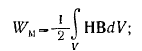
taking into account that B = rotA, we obtain

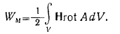
Using the identity

we obtain

Taking into account the second Maxwell equation in the first integral and the Ostrogradsky—Gauss theorem in the second integral, we find

Next we take into account that steady currents are closed and, substituting , we transform the first integral to the form

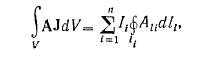
where n is the number of closed currents. Let us use the relation.

where Φi is the magnetic induction flux passing through the area S/ of the i-th current loop.
The second integral must be taken over a closed surface
of very large dimensions, so that it encompasses all the currents. Since 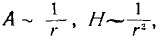, and the surface , the surface integral is equal to zero.
As a result we find
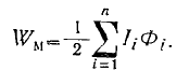(1)
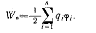
We note that this expression is analogous to the formula for the energy of a system of discrete charges

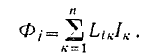
Expression (1) can be represented in another form by introducing the mutual inductance coefficient defined by the formula

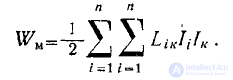
Substituting this expression into (1), we find

Owing to the fact that

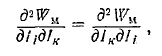
we obtain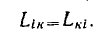
In particular, for a single loop

and

2. Stationary field

A field arising in a conductor carrying a steady current is called a stationary field.

Maxwell's equations for this field

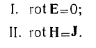
These equations must be supplemented with a constitutive equation — Ohm's law in differential form:

The equations written out reduce to Kirchhoff's laws of circuit theory. Indeed, the second Maxwell equation gives

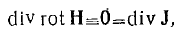
from which we immediately obtain Kirchhoff's first law

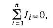
i.e., the sum of the currents at a node of wires is equal to zero (Fig. 1).

From the first Maxwell equation it follows that the stationary electric field is potential, since

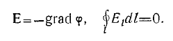
Substituting under the integral

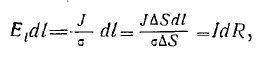
where

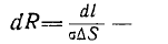
is the resistance of a wire element of length dl, we obtain

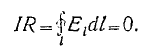
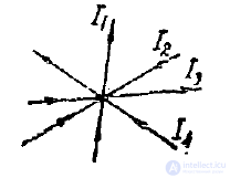
Fig. 1

Since , then I = 0, that is, a steady current cannot exist due to a stationary electric field alone.
It remains to assume that it is produced by an extraneous EMF, whose field intensity is .

Consequently, here Ohm's law must be generalized to include the intensity of the extraneous EMF field, that is
.
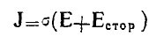Integrating both sides of this relation over a closed loop, we find

As a result we obtain from this Kirchhoff's second law


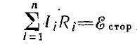
that is, the sum of the voltage drops across the individual sections of a closed circuit is equal to the extraneous EMF acting in that circuit (Fig. 2).

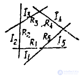
Fig. 2

3. Quasi-stationary field

A quasi-stationary field occurs in conductors carrying an alternating current that varies sufficiently slowly.
Criterion of slowness: the displacement current must be significantly smaller than the conduction current, that is

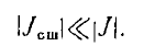
Accordingly, the quasi-stationary field is described by Maxwell's equations:

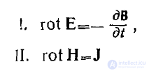
and two constitutive equations

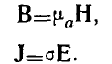
The equations written out reduce to Kirchhoff's laws for alternating currents.
Indeed, from the second Maxwell equation, as in the case of the stationary field, it follows that div J = 0 and, consequently, the first Kirchhoff law is applicable here without any modifications.
Further, the first Maxwell equation means that

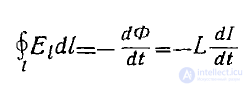
Thus, from everything considered in this lecture and earlier, it follows that there are three types of electric field intensity:

E — potential; for this field 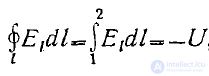, where U is the potential difference;

E — vortex or induced; for this field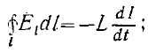
E — extraneous; for this field -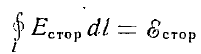

Taking these three types of fields into account, the generalized Ohm's law in differential form must be represented as
,
from which

i.e.

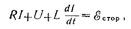
or

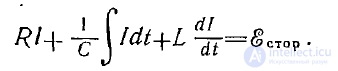
This is Kirchhoff's second law for alternating currents.

• Static electricity
• Electrostatic potential
• Electric field