SPHERICAL WAVES: Vector and Scalar Wave Equations in Spherical Coordinates

A spherical wave is a wave whose front is a sphere.

The phase-velocity vector of a diverging spherical wave is oriented radially outward from the source ("the wave radially diverges from the source"), while for a converging wave it is oriented toward the source. A spherical wave is a convenient model; in reality the wave front differs from a spherical one because of the properties of the source and the inhomogeneity of space. In the far zone of the source, a quasi-spherical wave of the optical range is formed, for example, by a small incandescent lamp, and of the radio-frequency range, by an antenna.

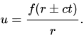
For a scalar wave the equation has the form

(1.2)

For a wave diverging from the oscillator, the sign − is used instead of ± in formula (1.2), and for a converging wave, +. Such a wave satisfies the wave equation, and the superposition of a converging and a diverging wave (in particular, a standing spherical wave as well) is also a solution of the wave equation.

The function f, generally speaking, can be arbitrary, but the case of a harmonic f can be singled out.

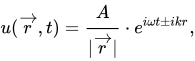
A harmonic symmetric spherical wave in a non-absorbing medium is given by the equation

(1.1)

where r is the distance from the source to the point of interest;

is the decreasing amplitude of oscillation;

ω is the angular frequency;

i is the imaginary unit;

k is the wave number;

the sign '—' corresponds to a diverging wave, and the sign '+' to a converging one.

If the quantity specifies the disturbance at a given point and at a given moment in time, then over a certain interval of time the energy carried away is But since the area of the sphere grows as, the flux of the function remains unchanged.

SPHERICAL WAVES
In the preceding chapter it was shown how the analytical difficulties^
associated with treating a vector differential equation in
curvilinear coordinates could be overcome in the cylindrical coordinate
system by resolving the field into two partial fields, each of which can
be obtained from a ^scalar function satisfying the wave
equation. Fortunately, this device is also applicable in spherical coordinates,^
to which we now turn. The special advantages of cylindrical and
spherical coordinates are a consequence of the simplicity of their geometric
properties. A deeper insight into the essence of the task before us»
and into the difficulties that arise when passing to curvilinear
coordinates in the general case, we shall obtain by first briefly studying
the vector wave equation.!^
THE VECTOR WAVE EQUATION
7.1. The fundamental system of solutions. Within a closed
region from which all sources have been removed and which is filled with a homogeneous
isotropic medium, all vectors characterizing the electromagnetic field,
namely the field vectors E, B, D and H, the vector potential and the Hertz vector,
satisfy one and the same differential equation. If we denote by
C any one of these vectors, this equation has the form:
By virtue of the linearity of this wave equation, a field varying arbitrarily
in time can be built up from harmonic solutions, and we shall not
diminish generality if we assume that the vector C contains time only
as a factor e-**"*. By the operator A acting on a vector, we
must understand AC = grad div C — rot rot C; therefore instead of A) we write
grad div C — rot rot C + k^2C = 0, B)
where, as usual, k^ = eμω^ + iσωμ.
The vector equation B) can always be replaced by the corresponding
system of three scalar equations, but resolving this system with respect to
any one of the components of C turns out in most cases to be practically
impossible [see (85), p. 55]. Only in the case when we
resolve C into three rectangular components do we obtain three independent
equations
AC_j + k^2C_j = 0, (j = x, y, z)
where the operator A can already be represented both in rectangular and
in curvilinear coordinates. Until now, very little attention has been paid to determining the independent vector^

solutions of equation B), but
recently such an attempt was undertaken by Hansen i) in a series of interesting
papers devoted to the study of antenna radiation.
Let the scalar wave function <^ be a solution of the equation
^^-^ψ = 0^ D)
and let a be some constant unit vector. We now construct
the following three independent vector solutions of equation B):
L = gradΨ, M = rot(aΨ), N=~rotM. E)
If in equation B) we set C equal to L, M or N, then equation B)
will be satisfied identically, provided that ^ satisfies
equation D). It is clear that, since a is a constant vector, we can write
M as
M = [L, a] = -|- rot N. F)
For one and the same generating function ^, the vector M is perpendicular
to the vector L, i.e.
LM = 0. G)
The vector functions L, M and N possess some remarkable
properties following directly from their definitions. The vector L is irrotational
and
rot L = 0, div L = ΔΨ = —k^2Ψ, (8)
the vectors M and N are solenoidal:
div M = 0, div N = 0. (9)
The particular solutions of equation D), finite, continuous and single-valued
in the given region, form a discrete system. Let us denote temporarily one
of these solutions by Ψ_n. With each of the characteristic functions
Ψ_n are associated three vector solutions of equation B), L_n, M_n and N_n, no
pair of which is collinear. It may be assumed that an arbitrary
wave function can be represented as a combination of
characteristic vector functions; the expansion coefficients can be determined,
since L_n, M_n and N_n possess orthogonality properties which we
shall prove later. If a given function is purely solenoidal, then it
can be represented as a combination of only M_n and N_n. If, however,
the divergence of the given vector function is not equal to zero, then the expansion
must also contain the functions L_n.
The vectors M and N are evidently suitable for representing the fields E and H,
since each of them is proportional to the curl of the other. Thus,
if time enters only as the factor e—iωt and if the density of
free charges is everywhere zero, then for a homogeneous isotropic medium with
conductivity σ we have
Let us now suppose that we can expand the vector potential in
characteristic vector functions in the form
A = -Σ(…a_nM_n + …+b_nL_n), (11)
n
E = ½ rot H, H=r½ rot E. - A0)
1) Hansen. Phys. Rev. 47, 139—143, January 1935; Physics 7, 460 — 465,

where the coefficients a_n, b_n and c_n must be found from the
distribution of currents.
According to (8), A0) and the relation μH = rot A, we obtain for the
field vectors
E = … Σ(a_nM_n + …N_n), H == … Σ(a_nN_n + …M_n). A2)
n n
The scalar potential does not play any role in the calculations, but obviously it can
be determined directly from A1), since according to B7), p. 36,
div A = -iωk^2φ; and consequently from (8)
φ = —Σ…Φ_n. A3)
U)
n
Thus, grad φ = —Σc_nL_n, and the relation
n
E = -gradφ—….
obviously again leads to formula A2). Finally, if we recall that
under these conditions the electromagnetic field can be expressed by means of two
Hertz vectors through the equations
E==rot rot Π+ iωμ rot Π*, H = …rot Π+rot rot Π*, A4)
then from this it becomes immediately clear that
Π = —Σ…a_na, Π* = —Σ…a_nΦ_na, A5)
n n
where a is a constant vector.
Before applying these results to the cylindrical and spherical
coordinate systems, we shall consider an elementary example of waves in
rectangular coordinates. A plane wave, whose wave vector equals
k = kn, can be represented in the form
Ψ=e^{ikR-iωt}, A6)
where R is the position vector drawn from a fixed origin. Since
kR = k_1x + k_2y + k_3z, it is easy to see that
L = ikK, M =ik[k, a], N = ik[[k, a], k]. A7)
In this particular case LM = MN = NL = 0; all three vectors are mutually
perpendicular and L is a purely longitudinal wave. Let α and β be the polar
angles determining the direction of the vector k, as shown in Fig. 66,
p. 319; the general solution of equation B) can be obtained by
integrating these plane-wave functions over all possible directions.
If g(α, β) is the scalar amplitude (weighting factor), then in some
coordinate system we can write for L, provided the conditions of
convergence
L = e^{-iωt} ∫dα ∫dβ g(α, β) k(α, β)e^{ikR} A8)
and similarly for M and N
M = e^{-iωt} ∫dα ∫dβ g(α, β) [k, a] e^{ikR}, A9)
N = e^{-iωt} ∫dα ∫dβ g(α, β) [[k, a], k] e^{ikR}. B0)

7.2. Application to cylindrical coordinates. The scalar characteristic
functions of the wave equation in cylindrical coordinates
were given in equation F), p. 315. The use of functions of the
complex angle exp (inθ) is associated with some inconveniences, and it turns out simpler
to use two real functions cos nθ and sin nθ, which we
shall denote simply as even and odd. The cylindrical wave
functions constructed from Bessel functions of the first kind and therefore
finite on the axis will be denoted by ψ_n^(1), while the wave functions
formed from H_n(λr) and H_n^(2)(λr) will be denoted respectively by ψ_n^(3) and ψ_n^(4).
Thus
ψ_{on}^{λ} = cos nθ J_n (λr) e^{ihz - iωt},
1.A) …
ψ_{en}^{λ} = sin nθ J_n (λr) e^{ihz - iωt},
ψ_{on}^{(2)λ} = cos nθ H_n^{(1)} (λr) e^{ihz - iωt},
ψ_{en}^{(2)λ} = sin nθ H_n^{(2)} (λr) e^{ihz - iωt},
B2)
where, as usual, λ = √(k^2—h^2) = k sinα. Functions of the first kind are expressed by
definite integrals of the form
2π
i^{-n}
J_{nλ} = … ∫ e^{iλR cos(β-θ)} cos nβ dβ e^{ihz-iωt},
0
2π
B3)
and the representations for functions of other kinds differ only in the choice of the path
of integration.
From B3) we shall now construct an integral representation for the vector
wave functions. Thus
1)'
1)
ψ_{en}^{λ} = grad ψ_{en}^{λ}
… , …
i_{en}^{λ}.
B4)
Differentiating B3) with respect to r, θ and z, and noting that λ sinα cos (β — θ),
λ sinα sin (β—θ) and h cosα are the components of the vector k relative to the
axes defined by the unit vectors i_r, i_θ, i_z, so that
k = i_rλ sinαcos(β—θ)+i_θλ sinα sin (β—θ)+i_z h cosα, B5)
we obtain for the even function the expression
1)'
215
l_{en}^{λ} = … ∫ k e^{iλR} cos (β-θ) cos nβ dβ e^{ihz-iωt},
0
B6)
which has the same form as A8). The corresponding expression for the
odd function is obtained by replacing cos nβ under the integral by sin nβ. In
applying these characteristic functions to expand an arbitrary vector wave
by them, it proves convenient to exclude the factor
1) The results of this section should be compared with equations C6)

exp(ihz — iωt), so we define the vector analogues of the scalar
function f(r, θ) (Chapter VI) by the relations
L—— 1 e^{ihz—iωt} … e^{ihz—iωt}
— e^{ihz-iωt}
From B6) we have
l_{en}^{λ}=… ∫ k e^{iλR cos(β-θ)} cos nβ dβ. B8)
2π
In the same manner we shall obtain integral representations for the
other independent solutions. If as the constant vector a we
take the unit vector i_z directed along the z axis, we find:
m_{en}^{(1)} = [grad ψ, i_z] = …
whence it is not difficult to obtain that
2π
0 0
And since rot m_n = n_n, we have
2π
n_{en}=… ∫ (i_zλ — ih k) e^{iλR cos(β-θ)} cos nβ dβ, B31)
0 0
Starting from these integrals, one can easily obtain also the rectangular
components of the wave functions. The vector function of the angle
appearing in the integrand is resolved into its rectangular components,
which may then be combined with cos nβ or with sin nβ. The resulting
scalar integrals can be computed by comparison
with B3).
In order that an arbitrary function of r and θ can be
expanded in the functions l_{en}, m_{en}, n_{en}, …, we must show that these functions
0 0 0
are orthogonal. Let i_r, i_θ and i_z be the unit basis vectors of the
circular cylindrical coordinate system (Fig. 7, p. 56), and Z_n(λr) be
the cylindrical Bessel function of any kind. Then, according to E), we
obtain
l_{en}^{λ} = i_rλZ_n' (λr) cos nθ i_1 + … Z_n (λr) sin nθ i_θ, C2)
m
sin , … , … cos
m_{en}^{λ}
… Z_n (λr) … nθ i_2 - … Z_n (λr) … nθ i_z, C3)
ih … , … … cos ihn … , … sin … … cos
n_{en}^{λ} == … Z_n' (λr) sin nθ i_1 =… Z_n' (λr) cos nθ i_2 + … Z_n (λr) … nθ i_3.
0
From these expressions it is at once evident that the integral from θ = 0 to 2π of
the scalar product of any two of these functions vanishes if
the indices n of these functions differ. Further:
∫ l_{onλ} l_{enλ'} dθ = ∫ l_{enλ} l_{enλ'} dθ = 0, if n≠n'. C5)

Let us understand by 1' the function l for which the sign of ih is reversed
… Then the normalizing factor can be found from
the integral
∫ l_{nλ} l_{nλ'} dθ = (1+δ) π r λZ_n(λr) λ'Z_n(λ'r) +
0
0 0
+ … Z_n (λr) Z_n (λ'r) + hh'Z_n (λr) Z_n (λ'r)] , C6)
where δ= 0 for n≠0, and δ=1 for n==0. The first two terms of the right-hand side
can be combined by means of the recurrence relations B4) and B5),
p. 317, which gives
∫l_{nλ}l_{nλ'}dθ = (1+δ)πr { λλ'[Z_{n-1}(λr)Z_{n-1}(λ'r) +
+ Z_{n+1}(λr)Z_{n+1}(λ'r)]+hh'Z_n(λr)Z_n(λ'r) } , C7)
The same recurrence relations also lead to the following integrals:
0 0 0 0
2π
∫m_{enλ}m_{enλ'} dθ = (1+δ) π r … [Z_{n-1} (λr) Z_{n-1} (λ'r) +
+ Z_{n+1}(λr)Z_{n+1}(λ'r)], C9)
2π 2π
0 0 0 0
2π
∫ n_{enλ}n_{enλ'} dθ = (1 + δ) π { … [Z_{n-1} (λr) Z_{n-1} (λ'r) +
0 0 0 …
+ … Z_{n+1}(λr)Z_{n+1}(λ'r)] + h^2 Z_n(λr)Z_n(λ'r)}. D1)
Moreover,
2π 2π 2π
∫ l_{enλ}m_{enλ'} dθ = ∫ m_{enλ}m_{onλ'} dθ = ∫ l_{enλ} n_{onλ} dθ = 0. D2)
0 0 0 0 0 0 0 0 0
and, using once again the same recurrence relation, we
obtain
2π 2π
∫ l_{enλ}n_{enλ'} dθ = ∫ m_{enλ}n_{enλ'} dθ = 0. D3)
0 0 0 0 0 0
Only one combination remains, which, unfortunately, leads to
a certain difficulty:
2π
∫ l_{enλ} n_{enλ'} dθ = (1 + δ) … { λλ'2Z_n (λr) Z_n (λ'r) —
— hh'[Z_{n-1}(λr)Z_{n-1}(λ'r) + Z_{n+1}(λr)Z_{n+1}(λ'r)] } , D4)

i.e. one obtains a quantity that does not vanish identically. Thus,
in view of D4), the system of vectors l_{en}, m_{en} and n_{en} is not completely
0 0 0
orthogonal with respect to θ. In many cases this is not essential, because,
if the divergence of the vector function is zero, as is the case
for the electromagnetic field vectors in the absence of free charges, then
it can be expanded only in m_{en} and n_{en}. But the complete expansion of the
0 0
vector potential requires the inclusion of the functions l_{en} also.
0
For the case of functions of the first kind, Hansen applied the Fourier–Bessel
theorem in order to obtain complete orthogonality and simplify the
expressions for the normalizing factors. After an obvious change of variables
we obtain from E3) and E4), p. 327,
∞ ∞
f(λ) ==∫rdr ∫λ'dλ' f(λ') J_n(λ'r) J_n(λr). D5)
0 0
We replace in C7), C9), D1) and D4) Z_n(λr) by J_n(λr) and apply
relation D5). Instead of f(λ') we shall have λ', h' ==√(k^2 — λ'^2), h'λ' etc.
It must be noted here that the validity of the Fourier–Bessel theorem
∞
was proved only for the case when the integral ∫|f(λ)|λdλ.
0
exists; in the present case this condition is not satisfied. The devices
which are used to ensure convergence are connected
with mathematical difficulties which lie beyond the scope of this book.
With some reservations we may introduce an exponential factor
ensuring convergence, as we did in the theory of the Laplace
transform on p. 276. Let us, accordingly, understand by 1(λ) the limit
0
to which l e^{-s|x|} tends as s→0. Then
0
∞ ∞
lim ∫ r dr ∫ λ' dλ' { λ'e^{-s|λ'|} } J_n(λ'r) J_n(λr) = … D6>*
Accordingly, the expressions for the normalizing factors take the form
∞ ∞ 2π
0 0 0 0 0
∞ ∞ 2π
∫∫∫ m_{enλ} J_{nλ'} λ' dλ'r dr dθ = (1+ δ) … D8>
0 0 0 0 0
* ∞ ∞ 2π
∫∫∫ n_{enλ} n_{enλ'}dθ = (1 + δ) …, D9>
0 0 0 0 0
1) The completeness of the system of vector functions has not been proved by us, but it may
be assumed on the basis of the completeness of the system of functions l_{enλ}.
0

whereas for the awkward expression D4) we obtain 1)
∞ ∞ 2π
0 0 0 0 0
THE SCALAR WAVE EQUATION IN SPHERICAL COORDINATES
7.3. Elementary spherical waves. Since an arbitrarily
time-varying field can be represented, by Fourier's theorem,
as a sum of harmonic components, we shall not diminish generality of
the results if we henceforth assume that
Ψ==f(R,θ,φ)e^{-iωt} A)
In a homogeneous isotropic medium the function f(R, θ, φ) must satisfy
the equation
Δf+k^2f=0, B)
which, according to (95), p. 57, has in spherical coordinates the form
The variables in this equation separate, so that, setting
f=f_1(R)f_2(θ)f_3(φ).
… + 2…+(…—p^2)f_1 = 0, D)
…+q^2f_3 = 0. F)
The parameters p and q, which are separation constants, are determined
from the physical requirement that the field be single-valued at any given point
of space; f_3(φ) must obviously be a periodic function of φ with period
equal to 2π, and consequently the range of possible values of q is restricted to
whole numbers m = 0, ±1, ±2, … To determine the parameter p, we
shall first show that the solution f_2 is identical with the associated Legendre
functions. After the substitution η = cos θ, equation E) takes the form
This equation has regular singularities only at the points η = —1,
η = +1 and η=∞. Its solutions will, therefore, be
hypergeometric functions. Further, for m = 0, G) reduces to Legendre's equation,
which has two independent solutions. Each of these solutions can be
expanded in a series of increasing powers of η in the neighborhood of η = 0. However,
in the general case these series do not converge at η= ±1. But if we take
p^2=n(n+1), where n = 0,1,2,…, then one of the series will terminate after a finite
number of terms and will have a finite value at the poles. These solutions
we obtain
1) It should be noted that the limit to which integral D6) tends as s → 0
is not necessarily equal to the value of the integral at s = 0, since the latter requires
continuity of the function defined by this integral in the neighborhood of the point s = 0.
This point lies at the basis of the whole theory of the Laplace transform. See, for example,
Carslaw, Introduction to the Theory of Fourier's Series and Integrals, 2nd ed.,
p. 293, Macmillan, 1921.

in the form of polynomials, satisfying the equation
{1-η^2}
… + n(n+1)w = 0,
(8)
are called Legendre polynomials and are denoted by P_n(η). If
(8) is differentiated m times with respect to η, we obtain
… d^w … d w
where w = d^n/dη^n. Making, finally, the last substitution of the dependent variable
m
w = (1—η^2)^{m/2} f(η), we obtain equation G) in the form
The solutions of equation A0), finite at the poles η = ±1 and, consequently,
periodic with respect to θ, will be the associated Legendre polynomials
dη^m
A0)
(11)
For each pair of integers there exists yet another independent solution
Q_n^m(η), which becomes infinite at η = ±1 and which,
consequently, is unsuitable for representing physical fields over the entire sphere.
The definition of the associated Legendre polynomials given in (11) has
meaning only for positive integer m and n. Functions with
negative indices are fairly simply related to functions with
positive indices, but we do not give them since we shall not need them.
To avoid any confusion on this point, we shall take
as particular solutions of F) the real functions cos mφ, sin mφ,
and restrict the values of m and n to positive integers or zero.
From (11) it is clear that for m>n the polynomial P_n^m(η) equals zero, since P_n(η) is
a polynomial of degree n. Indeed, we have
m
(1 — η^2)^{m/2} d^{n+m}(η^2—1)^n
P_n^m(η)
2^n n!
(12)
The Legendre functions are the most well-known example of
hypergeometric functions, whose properties have been studied in such detail
that it is hardly possible, within the space available to
us, to give any exhaustive account of the numerous integral representations of these functions
or of their series expansions.
We shall write out only the necessary recurrence relations:
(n—m+1)P_{n+1}^m —(2n+1)ηP_n^m+(n+m)P_{n-1}^m=0,
m
…
… m —1
P_{n+1}^m = ηP_n^m + (n+m)√(1-η^2)P_n^{m-1}
√(1-η^2)P_n^{m+1} = 2mηP_n^m —(n+m)(n—m+1)√(1-η^2)P_n^m
— 1
√(1-η^2)P_n^m=…(P_{n-1}^{m+1}—P_{n+1}^{m+1}±1).
m
√(1-
P_n^m=…[(n-m+1)(n+m)P_n^{m-1} + P_n^{m+1}]+
+m√(1-η^2)P_n^m.

To these we can add the differential relations:
1—
dP
(1-η^2)
dη
(n+m)P_{n-1}^m — nηP_n^m,
…=…=…{(n-m+1)(n+m)P_n^{m-1}—P_n^{m+1})
dη
(14)
Let us note in passing that the same relations are satisfied by the
functions of the second kind Q_n^m.
The functions cos mφ P_n^m(cosθ) and sin mφ P_n^m(cosθ) are periodic on the surface
of the unit sphere, and the number of nodal lines is determined by the indices m and n.
Thus, for m=0, the field is independent of the equatorial angle φ; if
n is also zero, then
the function is constant over the entire surface
of the sphere. For n = 1 there is
one nodal line, running
along the equator θ = π/2, along which
the function equals zero. For
n = 2 there are two nodal lines; they
run along the parallels
corresponding approximately to θ = 55°
and θ = 125°. Thus,
the sphere is thereby divided into three zones —
Fig. 69. Developed surface of the sphere, showing the nodes of the function sin 3φ P_5^3(cosθ). the function is positive in the
The shaded areas correspond to its negative values. polar zones and negative
in the equatorial zone. Continuing
in the same way further, we
obtain, evidently, that the number of nodal
lines equals n, and the number of zones, within each of which the function
retains its sign, equals n+1. Within each of the zones the function retains
its positive or negative sign. Therefore the functions P_n(cosθ)
are often called zonal harmonic functions. If now m
180°
180°
m
is different from zero, then, owing to the factor (1—η^2)^{m/2}, the function vanishes
at the poles, and the number of nodal lines parallel to the equator equals
n — m (see Appendix IV). In addition, the function vanishes also along
the meridians determined by the roots of cos mφ and sin mφ. Evidently there are m
meridional nodal lines, intersecting the latitudinal nodal lines at
right angles, and thus the surface of the sphere is divided into
rectangular regions or cells, within each of which the function
is alternately either positive or negative. The functions cos mφ P_n^m(cosθ) and
sin mφ P_n^m(cosθ) are therefore often called tesseral harmonic
functions of degree n and order m. Evidently there are 2n+1 tesseral
harmonics of degree n. Such a division of the sphere's surface
into positive and negative regions is shown graphically for the function
sin 3φ P_5^3(cosθ) in Fig. 69.
If the tesseral harmonic functions are multiplied by a system
of arbitrary constants and summed, we obtain a
surface spherical harmonic function of degree n, with which

we already dealt in Chapter III:
Y_n(θ, φ) == Σ(a_{nm} cos mφ + b_{nm} sin mφ) P_n^m (cos θ).
(15)
The tesseral harmonic functions form a complete system of functions,
orthogonal on the surface of the sphere 1). By integrating (12) by parts
it is easily shown that
+1
+1
dη
∫ P_n^m(η) P_{n'}^m(η) dη = 0, ∫ P_n^m(η) P_n^{m'}(η) … dη = 0
—1 —1
for n≠n' or for m≠m', respectively, and that
2 (n + m)!
(16).
∫[P_n^m(η)]^2 dη =
—1
+1
[P_n(η)]^2
dη
2n+1 (n —m)!,
1 (n + m)!
—1
m (n — m)!,
(17)
From these relations follows the fundamental theorem on the expansion of
an arbitrary function in a series of spherical harmonic functions: Let
g(θ,φ) be an arbitrary function on the surface of the sphere, continuous
together with all its first and second derivatives. Then g(θ,φ)
can be represented as an absolutely convergent series of
surface harmonic functions
∞
g(θ,φ)=Σa_{n0}P_n(cosθ)+
n = 0
n
+Σ(a_{nm}cos mφ+b_{nm}sin mφ)P_n^m (cosθ)], (18)
m =1
whose coefficients are determined by the relations
a
2n+ 1
2π π
n0
4π
∫∫ g(θ, φ) P_n (cos θ) sin θ dθ dφ,
0 0
a_{nm}…2… (n + m)!
2π π
∫∫ g(θ, φ) P_n (cos θ) cos mφ sin θdθ dφ
0 0
2π π
b_{nm} = … ∫∫ g(θ, φ) P_n (cos θ) sin mφ sin θ dθ dφ.
0 0
(19)
In the case of a function depending only on θ, the convergence conditions of the expansion
in Legendre polynomials coincide with the convergence conditions of a Fourier series.
In that case it suffices that the function g(θ) and its first
derivative be piecewise continuous in the interval 0 < θ < 2π. On the other hand,
the theory of convergence of the expansion (18) in spherical surface harmonics
1) A proof of this statement and of the following expansion theorem
can be found in R. Courant and D. Hilbert, Methods of Mathematical
Physics, M.—L., GTTI, 1933, Ch. VII, § 5. For further details see
Hobson, Theory of Spherical and Ellipsoidal Harmonics, Cambridge
University Press, 1931.

presents considerably greater difficulties, and the extension of the expansion
theorem to discontinuous functions lies beyond the scope of this survey.
It remains only to establish the character of the radial functions f_1(R),
_ 1_
satisfying equation D). If we write f_1 in the form f_1 = (kR)^{-1/2} v(R),
then it is easy to show that v(R) satisfies the equation
Consequently, according to section 6.5, v(R) is a cylindrical function
of half-integer order.
The characteristic or elementary wave functions, finite and
single-valued at all points on the surface of the sphere, will, therefore, be
Ψ_{mn}=…Z_{n+1/2}(kR)…P_n^m(cosθ)…cos mφ,
m   kR … sin mφ. (22)
As in the case of cylindrical waves, in the region including the origin
of coordinates, we take as Z_{n+1/2}(kR) Bessel functions of the first kind, and
where the field represents a traveling wave, functions of the third kind.
7.4. Properties of the radial functions. At various times different notations have been used for the radial
1
functions (kR)^{1/2}Z_{n+1/2}(kR), but none of
… + …
them has gained universal acceptance*). We shall follow
the notation which was recently proposed by Morse 2) and which
seems to us more or less logically justified. Accordingly
we define the spherical Bessel functions by the relations
…
(23)
The expansion of these functions in a series about the point ρ = 0 can be
obtained directly from (8) and (11), p. 315. If we recall that Γ(z+1) =
zΓ(z), Γ(1/2) = √π, and use the duplication formula, according to
which
we obtain for j_n(ρ)
∞
j_n(ρ) = √π/2 Σ (—1)^m (n + m)! ρ^{n+2m}, (25)
… / m!(2n+2m+1)!
m=0
1) See Watson, Bessel Functions, p. 55, Cambridge University

whence it is evident that j_n(ρ) is an entire function. In the same way, from
the relation N_{n+1/2}(ρ) = (—1)^{n+1} J_{-n-1/2}(ρ) for the function of the second kind
we obtain
∞
n_n(ρ) — Σ (—1)^m (n—m)! ρ^{2m-n-1} / m!(n-m+1)!, (26)
m = 0
Let us now turn to the representations for the case when ρ is a very large
number. On p. 316 the expansion in decreasing powers of ρ was given for
functions of arbitrary order p. Such series formally satisfy
Bessel's equation, but are only semi-convergent. However, as we
may note, for ρ = n+1/2 the series P_{n+1/2}(ρ) and Q_{n+1/2}(ρ) terminate,
2
so that the question of convergence does not arise at all. Correspondingly,
expressions (13) and (14), p. 316, will be analytic representations
of J_{n+1/2}(ρ) and N_{n+1/2}(ρ). It is evident, moreover, that these functions of half-
integer order can be represented as a finite number of terms.
From (23) and from equations (13) and (17), p. 316, we obtain that
j_n(ρ) = … { P_{n+1/2}(ρ) cos (ρ — (n+1)π/2) — Q_{n+1/2}(ρ) sin (ρ — (n+1)π/2) }. (27).
n_n(ρ) = … [P_{n+1/2}(ρ) sin (ρ — nπ/2) + Q_{n+1/2}(ρ) cos(ρ — nπ/2)], (28)
where
P_{n+1/2}(ρ) — 1 … 2ρ^2 …, (29)
Q_{n+1/2}(ρ) … 2ρ …. (30)
For functions of the third and fourth kind these expressions give
h_n^{(1)}(ρ) = i^{-n-1}e^{iρ} { P_{n+1/2}(ρ) + i Q_{n+1/2}(ρ) },
n+1
h_n^{(2)}(ρ)=i^{n+1}e^{-iρ}{P_{n+1/2}(ρ)—i Q_{n+1/2}(ρ)}.
(31)
These series converge very rapidly, so that for large ρ already the first terms alone
give sufficiently accurate values. Thus, as
ρ → ∞
j_n(ρ) ≈ … cos (ρ — (n+1)π/2), n_n(ρ) ≈ … sin (ρ — (n+1)π/2),
h_n^{(1)}(ρ) ≈ (—i)^{n+1}e^{iρ}/ρ, h_n^{(2)}(ρ) ≈ i^{n+1}e^{-iρ}/ρ.
(32),
The recurrence relations satisfied by the spherical Bessel
functions are obtained directly from equations (24)—(27),
p. 317:
Z_{n-1} + Z_{n+1} = (2n+1)/ρ … Z_n, (33).
… Z_n(ρ) = … { n Z_{n-1} — (n+1) Z_{n+1} }, (34)
d/dρ { ρ^{n+1}Z_n(ρ) } = ρ^{n+1}Z_{n-1}, d/dρ { ρ^{-n}Z_n(ρ) } = —ρ^{-n}Z_{n+1}. (35)

Having thus determined the radial functions, we can, finally,
write the general solution of equations C) in the form of a sum of elementary
spherical wave functions. In the case where f(R, θ, φ) must be
finite at the origin, we have
f^{(1)}(R,θ,φ)=Σj_n(kR)P_n(
n
n = 0
cos θ) + Σ(a_{nm} cos mφ +
m = 1
+b_{nm}sin mφ)P_n^m(cosθ)],
(36)
while the field whose surfaces of equal phase move
outward is expressed by the function f^{(3)}(R, θ, φ), obtained from (36) by replacing
j_n(kR) with h_n^{(1)}(kR). Spherically symmetric solutions are obtained in the
case when all coefficients, except a_{00}, are zero. Up
to an arbitrary factor we then obtain that
(1) sin kR
f_0 —
kR
(2) cos kR
f_0
…
kR
e^{ikR}
f_0^{(3)}
kR
e^{-ikR}
f_0^{(4)} =
kR
(37)
7.5. The addition theorem for Legendre polynomials. If g(θ, φ) is
some function satisfying the conditions of the expansion theorem (18),
then its value at the pole θ = 0 must equal
2π π
[g(θ,φ)]_{θ=0} = Σa_{n0}=Σ(2n+1)/4π ∫∫ g(θ,φ) P_n(cosθ) sinθ dθ dφ, (38)
n=0 n=0 0 0
+1…
since P_n(1)=1, P_n(—1) = 0. Let us take, in particular, as the
function g(θ,φ) some surface harmonic function of degree n,
Y_n(θ, φ), whose expression is given
by formula (15). Then, by virtue of the
orthogonality relations, the sum (38) reduces to
just one term, and we obtain
the following formula:
2π π
∫∫ Y_n(θ, φ)P_n(cosθ) sinθ dθ dφ
0 0
4π
= … [Y_n(θ, φ)]_{θ=0}. (39)
Fig. 70. On the addition theorem.
With the help of this formula we obtain
expressions for the transformation of zonal
harmonic functions when passing to a new
frame of reference. Let P in Fig. 70 be
a point on the sphere, whose coordinates in
the given orthogonal frame of reference are θ and φ. Let the coordinates of another point Q
be α and β, and let the angle between the axes QP and OQ be γ. The zonal
harmonic functions at the point P with respect to the new polar axis OQ
will have the form P_n(cosγ), and our task consists in expressing
P_n(cosγ) in terms of the coordinates θ, φ and α, β.
On the unit sphere cosγ is evidently equal to the projection of the line OP
on the axis OQ. If x, y, z are the coordinates of the point P, and x', y', z' the co-

ordinates of the point Q, then
cos γ == xx' +yy' + zz' = sinθ sinα cos(φ—β) + cosθ cosα, (40)
Let us assume that the desired expansion for P_n(cosγ) has the form
n
P_n(cosγ) = P_n(cosα)P_n(cosθ) + Σ(c_{nm}cos mφ + d_{nm}sin mφ)P_n^m(cosθ); (41)
m = 1
let us multiply both sides by P_n^m(cosθ)cos mφ and integrate over the whole
unit sphere. Using once again the orthogonality relations, we
obtain
∫∫ P_n(cosγ)P_n^m(cosθ)cos mφ sinθdθdφ = … c_{nm}. (42)
0 0
But, according to (39),
∫∫ P_n(cosγ)P_n^m(cosθ) cos mφ sinθ dθ dφ =
0 0
= … [P_n^m(cosγ)]_{θ=0} = … P_n^m(cosα) cos mφ, (43)
since at γ=0 we have θ=α, φ=β. Consequently,
Similarly
… = … P_n^m(cosα) sin mβ. (44>
The desired expansion, or addition formula, will therefore be
P_n(cosγ) = P_n(cosα) P_n(cosθ) +
n
m = 1
On the basis of this result we can give another expression for
the theorem stated on p. 355, namely: if g(θ,φ) and its
derivatives possess the required continuity properties on the surface
of the sphere, then Laplace's series (18) for this function will have the form
g(θ,φ)=ΣY_n(θ,φ), (47)
or, by virtue of (19) and (46),
n = 0
2π π
g(θ,φ)=…Σ(2n+1) ∫∫ g(α,β)P_n(cosγ)sinαdαdβ. (48)
n=0 0 0
7.6. Expansion of a plane wave. It is now comparatively simple to
obtain the expansion of a plane wave propagating in an arbitrary
direction, into elementary spherical waves about some
given center. The direction of propagation and the wavelength are determined
in the plane wave by the wave vector k, whose rectangular components
equal
k_1 = k sinαcosβ, k_2 = k sinα sinβ, k_3 = k cosα. (49

The coordinates of an arbitrary observation point will be
x = R sinθcosφ, y==R sinθsinφ, z = R cosθ. (50)
The phase of the wave is then determined by the expression
kR = k R [sinα sinθ cos(φ — β) + cosα cosθ] = kR cosγ. (51)
The function f^{(1)}(R, θ, φ) = exp(ikR cosγ) is continuous and has continuous
derivatives everywhere, including the origin R = 0. It may, therefore,
be expanded by formula (36), p. 358. Let us consider first of all
the axis whose direction coincides with the direction of propagation
of the wave. By virtue of the symmetry of the wave about this axis, we can write
that
∞
e^{ikR cosγ} = Σ a_n j_n(kR) P_n(cosγ), (52)
n = 0
The coefficients can be determined in the usual way, by
multiplying both sides of the equality by P_n(cosγ)sinγ and integrating with respect to γ from 0
to π. Then, taking (17) into account, we obtain
π
a_n j_n(kR) = … ∫ e^{ikR cosγ} P_n(cosγ) sinγdγ. (53)
0
In order to eliminate the dependence on R in this relation,
let us differentiate both sides with respect to ρ = kR and then set ρ = 0. Since,
according to (25),
[d^n j_n(ρ) / dρ^n]
_{ρ=0} = n! / (2n+1)!, (54)
π
0
The integral on the right is easily evaluated, and we obtain that a_n = (2n + 1) i^n, i.e.
∞
e^{ikR cosγ} = Σ i^n(2n + 1) j_n(kR) P_n(cosγ). (56)
n = 0 ,
… i.
If the z axis of the coordinate system does not coincide with the direction
of propagation of the wave, we can make use of the addition theorem (46),
in order to write (56) with respect to an arbitrary system
of coordinate axes. We then obtain
that
∞
e^{ikR cosγ} = Σ i^n(2n + 1)j_n(kR) [ P_n(cosα) P_n(cosθ)
n = 0
n
+ Σ … (n-m)!/(n+m)! P_n^m(cosα)P_n^m(cosθ)cos m(φ-β)}: (57)
7.7. Integral representations. We have found that in certain
cases it proves convenient to represent the wave function as a sum of
plane waves with corresponding weights or amplitude factors.
The direction of propagation of each of these plane components
is determined by the angles α and β. The integration must be extended over
all possible directions in space and may in some
cases include imaginary values of α or β. As in section 6.7, we

wish to find representations of the form
f(x, y, z) = ∫dα∫dβ g(α, β) e^{ik(x sinαcosβ+y sinαsinβ+z cosα)} (58)
or, if x = R sinθcosφ, y = R sinθsinφ, z = R cosθ,
f(R, θ, φ) = ∫dα∫dβg(α, β) e^{ikR cosγ} (59)
where α and β are the angles shown in Figs. 66 and 70. In the case of a cylindrical
wave, a constant frequency and a constant wavelength along the z axis lead
to a constant value of α, so that the directions of the plane waves
representing the cylindrical function f(ω, z) form a circular cone.
Since spherical waves have no such preferred direction,
the integration must be carried out over both α and β.
The integral representation of the elementary spherical wave
function can be obtained directly from the expansion (57). If both
sides of this equation are multiplied by P_n^m(cosα)cos mβ, or by P_n^m(cosα)sin mβ,
then, by virtue of the orthogonality relations (19), we obtain as a result
i^n j_n(kR) P_n^m(cosθ) cos, sin mφ = … ∫∫ e^{ikR cosγ} P_n^m(cosα) cos, sin mβ
… sinα dα dβ. (60)
0 0
After multiplying both sides by arbitrary constants a_{nm} and b_{nm} and
summing over m, this result can also be written as
2π π
i^n j_n(kR) Y_n(θ, φ) = … ∫∫ e^{ikR cosγ} Y_n(α, β) sinα dα dβ. (61)
0 0
From these general formulas one can obtain many useful expressions for
various special cases. Thus, for example, setting m = 0, β=0, we
obtain the representation for the spherical Bessel function j_n(kR)
π
j_n(kR) = … ∫ e^{ikR cosα}P_n(cosα) sinα dα, (62)
or
+1
—1
It is easy to show that the integral
j_n(kR) = … ∫ e^{ikRη} P_n(η) dη. (63)
z_n(kR) = i^{-n}… ∫ e^{ikRη} P_n(η) dη (64)
C
does indeed satisfy equation D), p. 352, provided that
the path of integration C is chosen so that the bilinear expression
(1—η^2)(dP_n/dη — ikRP_n)e^{ikRη}]_{…}^{…} = 0 (65)
vanishes at the limits of integration. Instead of η = ±1 we may
choose values at which the exponential factor
vanishes. Thus, if k is real, then as the upper limit we

may take η=—i∞ and obtain the following representations:
1 )
h_n^{(1)}(kR) = i^{-n} ∫ e^{ikRη} P_n(η) dη.
—i∞
i∞
h_n^{(2)}(kR) ==i^{-n} ∫ e^{ikRη} P_n(η) dη.
—1
(66)
If, because of the conductivity of the medium, k is complex, we may take that
root k such that its imaginary part is positive, and replace the limit η=i∞
by η = ∞.
From (60) and (54) we can obtain representations also for the functions
P_n^m(cosθ), setting φ and R equal to zero:
P_n^m(cosθ) = … ∫∫ cosγ… P_n(cosα) cos mβ sinα dα dβ. (67)
0 0
Carrying out the integration with respect to α by means of the
formulas at our disposal is difficult; it can, however, be shown by another route that
expression (67) reduces to the following:
P_n^m(cosθ) == … i^{-m} ∫ (cosθ+i sinθ cosβ)^n cos mβ dβ. (68)
0
Let us note, finally, that by using for the Bessel function the
integral representation (37), p. 323, one can reduce the right side of (60)
to a single integral. At m = 0
J_n(kR)P_n^m(cosθ)==
== … ∫ e^{ikR cosθcosα} J_m(kR sinθ sinα) P_n(cosα) sinα dα. (69)
0
7.8. The Fourier–Bessel integral. Let us assume that f(x, y, z) is
an arbitrary piecewise continuous function with piecewise continuous first
derivatives, and that the integral of the absolute value of this function,
extended over all space, exists. Then for this function
a Fourier integral exists
∞ ∞ ∞
f(x, y, z) = (…)^3 ∫∫∫ g(k_1, k_2, k_3) e^{i(k_1x + k_2y + k_3z)} dk_1 dk_2 dk_3, (70)
—∞ ∞ ∞
and the function transformed by Fourier with respect to f will be
3 ∞ ∞ ∞
g(k_1, k_2, k_3) = (…)^3 ∫∫∫ f(x, y, z) e^{-i(k_1x + k_2y + k_3z)} dx dy dz. (71)
—∞ ∞ ∞
Let us now transform these integrals to spherical coordinates,
tacitly assuming that the triple integral over an infinite cube may
be replaced by an integral over a sphere of infinite radius. Following the same
path as in section 6.9, and noting that k_1x+k_2y+k_3z=kR cosγ,

we obtain
3 ∞ π 2π
f(R, θ, φ) = (…)^3 ∫∫∫ g(α, β, k) e^{-ikR cosγ} k^2 sinα dk dα dβ, (72)
0 0
3 ∞ π 2π
g(α, β, k) = (…)^3 ∫∫∫ f(R, θ, φ) e^{-ikR cosγ} R^2 sinθ dR dθ dφ. (73)
0 0 0
Let us now assume that f(R, θ, φ) = f_n(R) Y_n(θ, φ). On the function
Y_n(θ), otherwise arbitrary, we impose the condition of
piecewise continuity together with its first derivative, and require the existence
∞
of the integral ∫|f_n(R)|dR. Then
0
3 ∞ π 2π
g(α, β, k) = (…)^3 ∫ R^2 dR f_n(R) ∫∫ Y_n(θ,φ)e^{-ikR cosγ}sinθdθdφ. (74)
0 0 0
This expression, by virtue of relation (61) and of the fact that j_n(—kR) =
= (—1)^n j_n(kR), becomes the following:
g
— …
g(α, β, k) = (—1)^n Y_n(α, β)√(…) ∫ f_n(R)j_n(kR)R^2dR, (75)
or g(α, β, k)=(—1)^n Y_n(α, β)g_n(k). Substituting this value for the
transformed function back into (72) and again changing the order of integration, we
find
— °°
f_n(R)Y_n(θ,φ)=… ∫ g_n(k)j_n(kR)k^2dk Y_n(θ,φ), (76)
0
whence we obtain yet another symmetric pair of mutually transforming
functions
∞
0
∞
g(k)=√(…)∫f(R)j_n(kR) R^2dR. (78)
0
The index n is omitted here, since it no longer has any
special meaning. In the particular case n = 0, equations (77) and (78) reduce
to the ordinary Fourier integral (18), p. 257. If the chosen value
of R coincides with a point of discontinuity of the function f(R), then we write
∞ ∞
… k^2dk ∫f(ρ)j_n(kρ)j_n(kρ')ρ^2dρ = ½[f(R+0)+f(R-0)]. (79)
0 0
7.9. Expansion of the cylindrical wave function. In calculating
the radiation of a given distribution of alternating currents it is sometimes
necessary to express the cylindrical wave function in spherical
coordinates. The integral representation for the wave function, finite

on the axis, will be
cos
sin
… J_m(λr) e^{ihz} = √(…) ∫ e^{iλR cos(β-φ)+ihR cosθ} cos, sin mβ dβ. (80)
…
0
Further,
kR = λr cos(φ — β)+hz = k{ sinα sinθ cos(β — φ)+cosα cosθ }, (81)
and on p. 360, formula (57), we have the expansion of the function exp(ikR) by
the corresponding spherical wave functions. Integrating with respect to β, we
obtain
… J_m(λr) e^{ihz} =
…
∞
= Σ i^{n-m}(2n + 1) … (n-m)!/(n+m)! P_n^m(cosα)P_n^m(cosθ)j_n(kR). (82)
n = 0
Since for m>n the polynomials P_n^m are zero, the first m terms in (82) are
zero, and the expansion can be written in the form
J_m(λr)e^{ihz} =
= Σ i^{n-m}(2n + 1) (n-m)!/(n+m)! P_n^m(cosα)P_n^m(cosθ)j_n(kR). (83)
n!
n=… (n+m)! …
If α = π/2, then h = 0, k = λ, and
…
0, if n is odd,
P_n^m(0)— { 1…, if n is even. (84)
2^{n+m-1}(…)!((n-m)/2)!
As a result we obtain the expansion of the cylindrical Bessel function
in a series of spherical Bessel functions
∞
Σ… 2^{l+2m} l!(l+m-1)! P_{2l+m}(cosθ)j_{2l+m}(kr). (85).
l=0
7.10. The addition theorem for the function Z_0(kR). Let P(R_0, θ, φ) be
the point of observation, and Q(R_1, θ_1, φ_1) the source of the spherical wave.
The coordinates R_0, θ, φ and R_1, θ_1, φ_1 are taken relative to a fixed system
of coordinates, with origin at the point O. The distance from Q to P
equals
R = √(R_0^2+R_1^2 — 2R_0R_1cosγ)
where cosγ = cosθ cosθ_1 + sinθ sinθ_1 cos(φ —φ_1). Our task consists in
expressing the spherical wave propagating from the point Q as a
sum of spherical waves whose source is located at the point O. The solution
of this problem in the general case requires lengthy calculations, and its
practical significance is not great enough to justify the expenditure of time and
space. However, in the theory of radiation we shall have an example of the application
of one special case of this theorem, namely the case of the transformation of a

wave, spherically symmetric with respect to the source Q. For this
case, without particular difficulty, one can obtain the following expansions:
∞
j_0(kR) = sin(kR)/kR = Σ(2n + 1)P_n(cosγ)j_n(kR_0)j_n(kR_1), (86)
n = 0
…
… e^{ikR}/kR
h_0^{(1)},
Σ(2n +1) P_n(cosγ)j_n(kR_0) h_n^{(1)}(kR_1) (R_0< R_1),
…: (87)
Σ(2n +1) P_n(cosγ) j_n(kR_1) h_n^{(1)}(kR_0) (R_0 > R_1).
n = 0
Their proof is left to the reader.
THE VECTOR WAVE EQUATION IN SPHERICAL COORDINATES
7.11. Spherical vector wave functions. As in the case of
cylindrical coordinates, one can obtain solutions of the vector
wave equation in spherical coordinates directly from the
characteristic functions of the corresponding scalar equation. Following the
notation of the preceding section, we set Ψ_e =Ψ e^{-iωt}, where Ψ is a
characteristic solution
According to section 7.1, one of the solutions of the vector wave equation
grad div C — rot rot C + k^2C = 0 (2)
can be obtained if we simply take the gradient of (1). We
define L as grad Ψ and separate off the time factor, setting L = l e^{-iωt}.
Then, according to (95), p. 57,
l_{mn} = i_1 Ψ_n P_n^m(cosθ) cos, sin mφi_1 + i_2 Ψ_n(kR) … P_n^m(cosθ) cos, sin mφi_2
… Ψ_n(kR) P_n^m(cosθ) cos, sin mφi_3, (3)
where i_1, i_2 and i_3 are the unit vectors shown for the spherical system
of coordinates in Fig. 8, p. 56.
In order to obtain the independent solutions M and N, we must,
in accordance with section 7.1, introduce a constant vector a. Such an
operation is, of course, admissible in the present case, but the functions M and N
obtained in this way will be neither normal nor purely tangential over the entire
surface of the sphere. Instead of a we shall use the radial vector i_r;
then the vector function [l, i_r] will be tangential over the entire surface of the sphere.
But i_r is not a constant vector, and we cannot, therefore, assert
a priori that we shall thereby obtain an independent solution. We shall show, however,
that the tangential solution M can indeed be constructed with
the help of the radial vector i_r. Unfortunately, this method is not applicable to more
general coordinate systems.
Let us try to construct a solution of equation (2) in the form of a vector
M = rot(i_r u(R)Ψ)=[l,i_r]u(R),

where u(R) is an unknown scalar function of R. Then, if M_R, M_θ and M_φ
represent the R-, θ-, φ- components of the vector M,
The divergence of M is zero, and we shall now resolve the equation rot rot M — k^2M = 0
into R-, θ- and φ-components by the formulas (85), p. 55. The R-component
is identically zero for any choice of u(R). The conditions for the θ- and
φ-components will be satisfied if u(R) satisfies the equation
… + … […u—k(…)] +
+…+k^2u=0. (5)
(A particular advantage of the spherical coordinate system compared with more
general systems is that this condition is the same for both
tangential components.) Consequently, if we take u(R) = R, then
relation (5) reduces to the required equation
…—k^2u = 0. (6)
…
Thus, in spherical

продолжение следует...

Продолжение:

Часть 1 SPHERICAL WAVES: Vector and Scalar Wave Equations in Spherical Coordinates
Часть 2 See also - SPHERICAL WAVES: Vector and Scalar Wave Equations