
Lecture
Up to now we have considered media with continuous variation of the parameters ε, μ and σ, for which all of Maxwell's equations hold in both integral and differential form. However, not all media have parameters that are continuous functions of the coordinates; abrupt changes in the medium's parameters are often encountered, for example at the interfaces between different materials. In that case Maxwell's differential equations turn out to be unsuitable at the boundaries, since the derivatives at these points have a discontinuity. Therefore the equations must be supplemented with boundary conditions, which relate the vectors on the boundaries of the media.
Boundary conditions make it possible to find the distribution of electromagnetic fields at the boundaries of various media, such as dielectrics, conductors, and vacuum. This is important for calculations in problems of electrodynamics and optics, and in the design of antennas or devices.
Maxwell's equations involve the vectors and sources of the
electromagnetic field. But the parameters of the medium do not
appear directly in them. Consequently, Maxwell's equations
hold for media with any parameters, including at the
interface between different media. However, at the boundary these equations
take on a special form — they are formulated as
boundary conditions. It is these boundary conditions that we now wish to obtain.
If the medium is homogeneous, then on an imaginary surface
inside the medium both the normal and the tangential components
of the field vectors will vary continuously when crossing
this surface.
If, however, this is a boundary surface between two media with
different electrical parameters, then it does not follow from anywhere
in advance that these components will vary continuously. A priori
it is unclear which components of the field vectors must vary
continuously, and which components may undergo a jump (a discontinuity
in continuity).
To obtain an answer to these questions, we will make use of the
fact that in reality there is no sharp boundary between
two different media with different electrical parameters.
There is a transition layer of some thickness, inside
which the electrical parameters vary continuously from their
values in one medium to their values in the other medium. Therefore
inside the layer, as well as outside it, Maxwell's equations hold.
We will obtain the sharp boundary, and likewise the formulation of Maxwell's equations
at the boundary, i.e., the boundary conditions, by means of a limiting
transition.
So, let the ox axis be perpendicular to the transition layer, and let
the curve in Fig. 1 represent the variation of some
electrical parameter on passing from medium I to medium II.
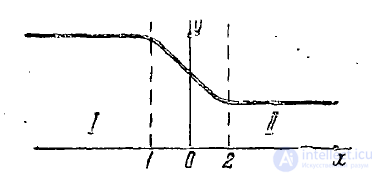
Fig. 1
Let us write the third Maxwell equation in the form
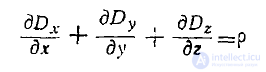
and integrate both sides of this equation over the range from point 1 to point 2 (Fig. 1).
We then obtain

or, considering the transition layer sufficiently thin, we find

The derivatives 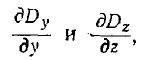 — and since they represent the changes of the quantities Dy and Dz in a plane parallel to the boundary plane — must be finite, so as
  we obtain where ps is the surface charge density, equal to

where 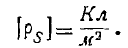
We see that Maxwell's equations allow for the existence of surface
charges, and their density must be determined by formula
(1).
Directing the normal n to the boundary plane along the ox axis, we can
write the boundary condition for the vector D as
 (2).
(2).
if surface charges are present, and
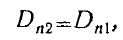 , (3)
, (3)
if there are none on the boundary surface.
The normal component of the electric displacement vector
undergoes a jump equal to the surface charge density when crossing the interface between two media,
or varies continuously,
if there are no surface charges.
In exactly the same way we can obtain the boundary
condition for the vector B:
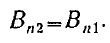 (4)
(4)
The normal component of the magnetic induction vector
varies continuously when crossing the interface between two media.
Let the transition layer be as shown in Fig. 1. Let us write
the second Maxwell equation as three scalar equations
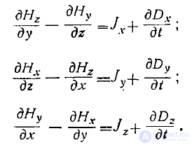
Let us integrate the last two equations over the range from point
1 to point 2 and obtain
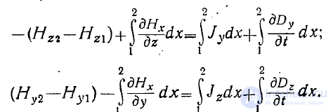
Considering the transition layer sufficiently thin, we obtain
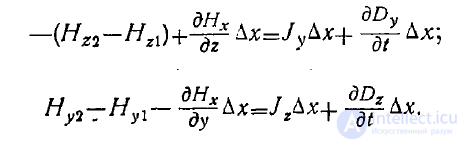
The derivatives 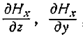 , since they represent
the changes of the quantity H in a plane parallel to the boundary plane,
dDy ÖD
are finite, as are —^- and , so as Δx→0 we obtain
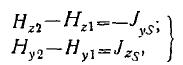 (5)
(5)
where Jy = y°JyS 4- z°JzS is the surface current density vector,
defined by the equalities
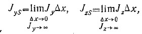 x, (6)
where [Jo] = 4 -
Δy→0 Δx→0
J y » -→0 y2-»-ao
We see that Maxwell's equations allow for the existence of
surface currents, and their density must be determined by formulas
(6).
Directing the normal n to the boundary plane along the ox axis, from boundary
condition (5) we obtain
 , (7)
, (7)
if surface currents are present, and
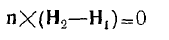
or, taking the vector t tangential to the interface,
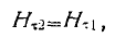 (8)
(8)
if there are none on the boundary surface.
The tangential component of the magnetic field intensity vector
undergoes a jump equal to the surface current density when crossing the interface between two media,
or varies
continuously, if there are no surface currents.
In exactly the same way we can obtain the boundary
condition for the vector E:
 . (9)
. (9)
The tangential component of the electric field intensity
vector
varies continuously when crossing the interface between two media.
Inside an ideal conductor (σ = ∞), as follows from the relations

the field is equal to zero. Since the corresponding field components
undergo a jump when crossing the surface of an ideal conductor, surface charges and currents must appear,
such that  , where
 (10)
(10)
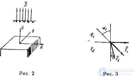
In this case the tangential component of the electric
field and the normal component of the magnetic induction are equal to zero
(Fig. 2).
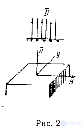
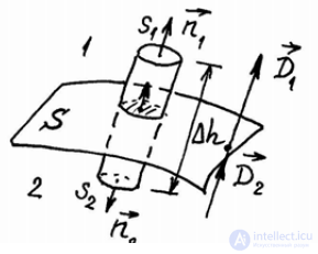
Figure 3.1
When considering the boundary conditions, the problem is posed as follows: let some surface S separate two regions of space with parameters (ε1, μ1 and σ1) and (ε2, μ2, σ2). In the vicinity of
the surface point under consideration, let us isolate a cylindrical volume of height Δh (Fig. 3.1) so that its axis
runs along the normal to the interface between the media, and let us consider the fluxes of the electric field
induction vector  through the surface of the cylinder.
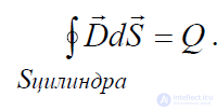
.
Let us identify three characteristic regions on the surface of the cylinder: the lateral
surface S_side, and the bases S1 (upper) and S2 (lower). In accordance
with this, the last equality can be written as:
 . (3.1)
We shall assume that the diameter of the cylinder is so small that within
both of its bases S1 and S2 the electric field induction Dr
can be considered constant. If we let the height of the cylinder Δh tend to zero (Δh →0), then
the integral over the lateral surface on the left-hand side of the last equality will also
tend to zero 0
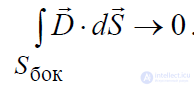
. In addition, S1 and S2 will move indefinitely closer together and in the limit will merge with each other, i.e.
S1 → S2 → S, and their outward normal vectors will be related as:
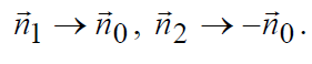
Taking the assumptions made into account, equation (3.1) can be reduced to the following form:

from which it follows:
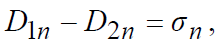 (3.2)
(3.2)
where 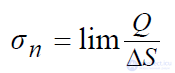
If  , then
 . (3.3)
Similarly, from equation 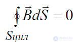 we find
 . (3.4)
We have examined how the normal components of the field vectors behave at the interface between two media.
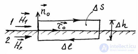
Figure 3.2
Let us now consider the behavior of the tangential field components at the interface, for which we mark out a loop L at the interface and consider the circulation of the vector H
r
around this chosen
loop. Let us write the 1st Maxwell equation in the form:
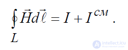
.
We shall assume that the dimensions of the loop L are so small that within
it the magnetic field intensity H
r
can be considered constant. Then
the left-hand side of this equation can be expanded as follows:

.
Now let us expand the right-hand side of the equation, for which we express the conduction current I and the displacement current I disp, passing through the cross-section of the loop,
in terms of their densities. Here two cases can be distinguished:
- the conduction current is volumetric, then

- the conduction current flows over the interface between the two media (surface current)

Equating now the left- and right-hand sides of the equation, we have:

Passing to the limit as Δh→0, we obtain
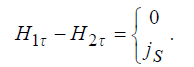 . (3.4)
Similarly, considering the circulation of the electric field
intensity E
r
around the loop L and applying the 2nd Maxwell equation, we can find the boundary
conditions for the tangential components of the electric field:
 . (3.5)
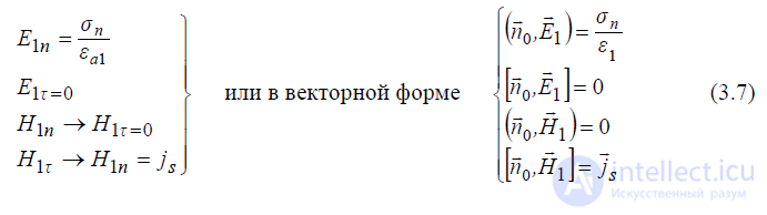
More rigorously, the complete system of boundary conditions can be written in vector
form:
 (3.6)
(3.6)
For time-varying fields, the boundary conditions on the surface of metallic bodies are considerably simplified, since here  is assumed.
Since the current density must be a bounded quantity, it follows from  that E ≡ 0. Setting E ≡ 0 in the 2nd Maxwell equation, we obtain = 0
 since the fields are time-varying, this last equality holds only when B ≡ 0.
Thus, in a perfectly conducting medium the fields are identically zero (i.e., they do not penetrate into the medium). If we assume the 2nd medium to be perfectly conducting, the boundary conditions are written as
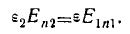
According to boundary condition (3) we can write
Taking boundary condition (9) into account
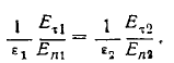
Denoting
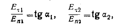
where  are the angles between the line perpendicular to the interface and the vectors E1 and E2 in the first and second media (Fig. 3),
we obtain
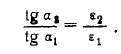 (11)
(11)
Similarly, using boundary conditions (4) and
we find
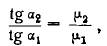 (12)
(12)
where  are the angles between the line perpendicular to the interface and the vectors H1 and H2 in the first and second media.
If we consider that of the two adjoining media, the one with the larger ε is electrically "denser," then from formula (11) it follows that the electric field vector lines move away from the perpendicular to the interface when passing from the less dense into the denser medium. A similar conclusion can be drawn on the basis of formula (12) regarding the magnetic field vector lines.

Comments