
Lecture
A plane wave — is a wave whose surface of constant phase is a plane.
The front of a plane wave is unbounded in size, and the phase-velocity vector is perpendicular to the front.
A plane wave is a particular solution of the wave equation and a convenient theoretical model: such a wave does not exist in nature, since a plane wave front would begin at −∞ and end at +∞, which obviously cannot be. Such a wave would carry infinite power, and infinite energy would be required to create it. The convenience of the plane-wave model is due to the fact that a wave with a complex (real) front can be represented as a superposition (spectrum) of plane waves by means of a Fourier transform over the spatial variables.
A quasi-plane wave — is a wave whose front is close to planar within some bounded region. If the dimensions of the region are sufficiently large compared to the characteristic size of the phenomenon, the quasi-plane wave can be approximately considered plane. A wave with a complex front can be approximated by a sum of local quasi-plane waves whose phase-velocity vectors are normal to the real front at each of its points. Examples of sources of quasi-plane electromagnetic waves are the laser, and reflector and lens antennas: the distribution of the electromagnetic field phase in a plane parallel to the aperture (the radiating opening) is close to uniform. As the distance from the aperture increases, the wave front takes on a complex shape.
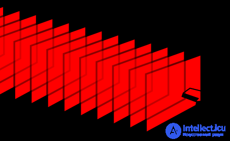
Fronts of a plane wave in three-dimensional space and the phase-velocity vector
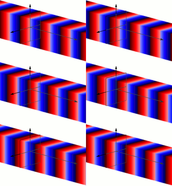
Animation of the motion of a plane wave
By definition, a plane electromagnetic wave is
a solution of the system of Maxwell's equations in which the vectors of the electromagnetic
field depend on only one coordinate of a rectangular
coordinate system. Let this be the coordinate z.
It is important that under these conditions Maxwell's equations admit
an exact solution.
Here and in what follows we will assume that the variation of the field
quantity in time occurs according to a harmonic law, and, consequently,
the time dependence will be represented by the factor
e-''"'. We will consider the medium to be homogeneous. Under these last two
conditions, in the absence of charges, Maxwell's equations III and IV
are, as follows immediately from the identities
c l i v r o t E ^ O , divrotHsO,
a consequence of the first two equations.
Thus, we can obtain the formulas for plane waves in a homogeneous medium
by operating only with the first two of Maxwell's
equations
The equation of any wave is a solution of the differential equation called the wave equation. The wave equation for a function A is written in the form
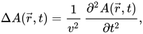
where Δ — is the Laplace operator;
 — is the sought function;
r — is the radius vector of the sought point;
v — is the wave speed;
t — is time.
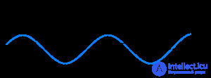
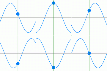
In this animated image, the horizontal axis represents the coordinate x in space, and the vertical axis represents the value of some oscillating physical quantity A , forming a wave with a harmonic time dependence, at each point in space at the current moment. The blue line — is the graph of the spatial dependence A(x) of the physical quantity at the current instant t=t1,t2,... The dependence on the coordinate is also harmonic. Shifting to the right over time, the graph A(x) coincides with itself at the previous instant — this is the wave process. The blue circle depicts the oscillation A(t) of the physical quantity A at one of the points along the coordinate 
In the one-dimensional case, the wave equation takes the form:
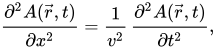
where x — is the coordinate.
A particular solution of this equation for a plane harmonic wave:

where A(x,t) — is the magnitude of the disturbance at the given point in space x and at the moment of time t ;
Ao — is the amplitude of the wave;
k — is the wave number;
ω — is the angular frequency;
φ0 — is the initial phase of the oscillation.
The wave number is expressed as:

where λ — is the spatial period of the function's variation, the wavelength.
The angular frequency of the oscillation is expressed as:
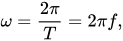
where T — is the period of oscillation;
f — is the frequency of oscillation.
Substituting these expressions into the expression for the wave, the wave can also be described by the expressions:
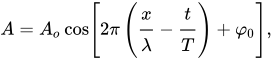 or:
or:
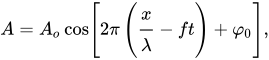 or:
or:
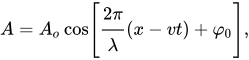
where v — is the phase velocity of wave propagation.
In the general case the equation of a plane wave is written in the form:

where  — is the wave vector, equal to
 — is the wave number;
 — is the unit normal vector drawn to the wave front;
 — is the radius vector of the point,
  — is the scalar product of the vectors and →.
The equations given above can be written in the so-called complex form:

or, in the multidimensional case:

The correctness of this formula follows from Euler's formula for the exponential with a complex exponent.
Generally speaking, the function can be either a real or a complex function. But since complex numbers do not exist in our real world, calculations that have finite physical meaning always reduce to computing either the real part, or the modulus, or the product of a pair of complex conjugates of this function.
From the complex notation of the harmonic function also follows the notion of the complex amplitude, equal to 
Then 
The modulus of the complex function gives the amplitude of the oscillations, and the argument — the initial phase φ0.
The exponential form of notation is often more convenient than the trigonometric one in some cases.
The most common notation:  .
.
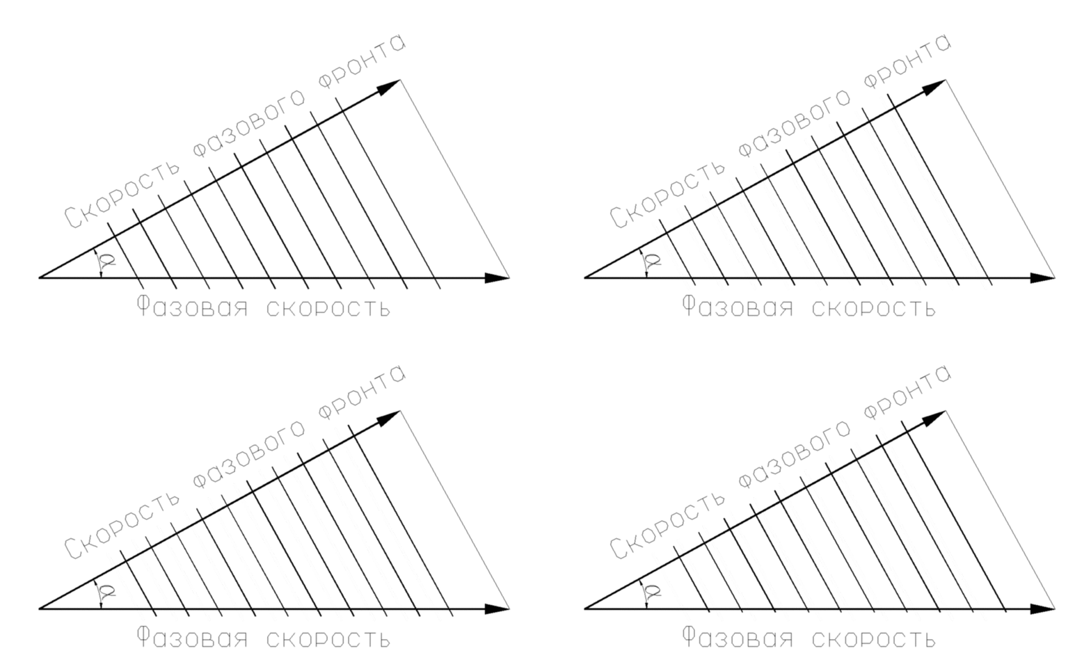
Phase velocity along a direction deviated from the wave vector by an angle α. A monochromatic plane wave is considered
Group velocity — is a quantity characterizing the propagation speed of a «group of waves» — that is, a more or less well-localized quasi-monochromatic wave (a wave with a sufficiently narrow spectrum). It is usually interpreted as the speed of displacement of the maximum of the amplitude envelope of a quasi-monochromatic wave packet (or wave train). When considering wave propagation in a space of dimension greater than one, it is usually understood to mean a wave packet close in shape to a plane wave.
In many important cases, the group velocity determines the speed of transfer of energy and information by a quasi-sinusoidal wave (although in the general case this statement requires serious refinements and reservations).
The group velocity is determined by the dynamics of the physical system in which the wave propagates (the specific medium, the specific field, etc.). In most cases the linearity of this system is assumed (exactly or approximately).
For one-dimensional waves the group velocity is calculated from the dispersion law:
 ,
,where  — is the angular frequency, — is the wave number.

Suppose that 
Let us isolate in space a certain small volume ΔV , small enough that at all points of this volume the particle velocity  and the strain
  can be considered constant.
Then the volume under consideration possesses kinetic energy:
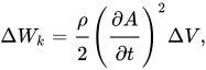
and potential energy of elastic deformation:

Total energy:

The energy density, respectively, is equal to:

One of the most important results obtained by Maxwell – the proof of the wave nature of the electromagnetic field (EMF).
Waves are disturbances that propagate with a finite speed in space and carry energy with them without the transport of matter. The wave process is one of the manifestations of the general regularity formulated as the so-called theory of contiguous action (near-action), according to which
any interaction can only be carried out sequentially from one point of space to another, and there is no such thing as instantaneous transmission of an interaction between distant points.
If some time process at point A changes according to the law f (t) , and at
point B, located at a distance r from A, this process changes as f (t) ,
then it is said that the function ( )
υ
f t − r describes a wave. Here υ – is the speed of
propagation of the wave, and the quantity τ = r υ determines the delay time
of the process at point B compared to point A. If the disturbance changes over
time according to the law of harmonic oscillations, then the wave process as a whole can be described by the function
=
υ
( − ) = Acosω(t − r )
v
f t r Acos(ωt − kr),
where the coefficient k = ω υ is called the wave number. Any waves
propagating in space are created by wave sources. The lines
along which waves propagate are called rays. If one connects
all the points that the wave has reached in the time Δt that has elapsed since some initial reference time t1, one obtains a surface, which is called the wave front. For a harmonic wave, its front is also a surface of equal phases. The path traveled by a harmonic wave during a period of oscillation
is called the wavelength λ = υ⋅T = υ f .
By the shape of the wave front, waves are classified as plane, cylindrical,
spherical. If the wave has the same amplitude at all points of the front, it is called homogeneous, otherwise – inhomogeneous.
In order to investigate the wave nature of the EMF, let us reduce Maxwell's equations to wave equations. To do this, consider a homogeneous unbounded medium with parameters ε , μ , with no sources of the electromagnetic field, for which the system of Maxwell's equations has the form:
rot , H E & r
& r
rot = − jωμ , (7.1)
0 div = D& r
, 0 div = B& r
. (7.2)
Let us apply the rot operation to the left and right sides of the first two of Maxwell's
equations:
E H & r
& r
rot j rot rot ε ω = , H E & r
& r
rot rot = − jωμrot .
Let us transform the resulting expressions, making use of the identity
(B.23) A A A
r r r
rot rot = graddiv − Δ and taking into account equations (7.2), as a result of which we arrive at the equalities:
E H & r
& r
rot jωε = Δ − , H E & r
& r
− Δ = − jωμrot .
Substituting now here E& r
rot and H& r
rot from (7.1), we obtain two identical
equations with respect to the vectors E& r
and H& r
:
0 2 = + Δ H k H & r
& r
, 0 2 = + Δ E k E & r
& r
, (7.3)
where k = ω εμ – is the complex wave number, which can be represented in
the form: k = β − jα, here β – is the phase constant, α – is the attenuation constant.
The differential equations in partial derivatives of the 2nd
order obtained are called the Helmholtz equations, or more often the wave equations.
Properties of the wave equations:
1. For an unbounded medium without sources, the wave equations are equivalent to the system of Maxwell's equations.
2. Equations (7.3) for E& r
and H& r
are identical in form, so the solutions of these
equations will also be identical in form.
3. The wave equations are written in complex form and are valid for monochromatic fields, so their solutions will be functions only of
coordinates.
4. The use of the wave equations instead of the system of 4 of Maxwell's
equations makes it possible to significantly simplify and shorten the solution of the problem
of finding E& r
and H& r
– in this case a system of three, instead of 12,
scalar equations is solved.
Since both equations (7.3) have solutions of the same form,
let us consider one of them, namely 0 2 = + Δ E k E & r
& r
. The general solution of this equation
in a Cartesian coordinate system is represented by the sum of two particular
solutions:
k r
m
k r
E Eme E e
r r r r
& r
& r
& r
= + − j + − j , (7.4)
where = β − αr r r
k j – is the wave vector, whose modulus is the wave number, and whose direction coincides with the direction of wave propagation; rr – is the radius
vector of the observation point.
Each of the two particular solutions (7.4) describes a wave. Let us prove this,
by writing the instantaneous value of the vector E& r
for the first solution
= { }=
= + − ω + −αr − βr ωt
m
kr t
E t Em e e E e e e j j
0
j j
( ) Re 0 Re
r r rr r r r r r
p Em(r ) cos( t r )
r r r r = ⋅ + ω + ϕ − β , (7.5)
where p r – is the unit vector indicating the initial direction of the vector E
r
;
+
0 m E – is the amplitude of the vector E
r
at the point r = 0 , taken as the origin;
r
Em r Em e
r rα
+ = + − 0 ) ( – is the amplitude of the vector E
r
at the current observation point;
e r
r rα
− – is the factor determining the exponential decrease of the amplitude (attenuation) of the oscillations with increasing r; hence α – is the attenuation coefficient;
ϕ and t rr rβ
Φ = ω + ϕ − – are the initial and current phases of the harmonic oscillation
respectively.
Let us consider the distribution of the electromagnetic wave field along the direction of its motion, assuming that α = 0 , ϕ = 0 and the vectors rr and β
r
are parallel.
In this case
E(t, r) = Em+0 cos(ωt − βr) (7.6)
and the distribution E(r) for a fixed instant of time t is a multi-extremal function, having the form of a cosine curve with maxima at
points rn , at which Φ = ωt − βrn = 2πn , n – an integer. The positions of these
maxima are determined by the expression:
rn = ωt /β + λn = υt + λn, (7.7)
where υ = ω β.
From (6) it follows that rn increases with increasing t, that is, over time the maxima of the distribution E(r) (the wave crests), and with them the entire wave,
will move along the r axis in the positive direction with a speed
υ. A wave possessing this property is called a traveling wave, and the exponential factor e r
r vβ
− j is called the traveling-wave factor.
Let us consider this factor in more detail, for which we express the vectors β
r
and
rr in terms of their projections in a rectangular coordinate system:
β = exβx + eyβ y + ezβz = ex cosϕx + ey cosϕy + ez cosϕz r r r r r r r
,
r ex x ey y ez z
r r r r = + + ,
whence
e j r e j( x x y y z z) e j (x cos x y cos y z cos z ) − β⋅ = − β +β +β = − β ϕ + ϕ + ϕ
r r
, (7.8)
where x ϕ cos , x ϕ cos and x ϕ cos – are the direction cosines of the vector β
r
.
The resulting expression (7.8) is convenient for describing electromagnetic waves propagating in an arbitrary direction β
r
, given
in a Cartesian coordinate system by its direction cosines.
The second particular solution differs from the first in that the sign before rr vβ
in
the exponent of the traveling-wave factor e r
r vβ
+ j is positive. It is easy to
show that the second term in (7.7) also represents a traveling electromagnetic wave, moving with speed v , but in the direction opposite
to the previous one, that is, toward negative r. In unbounded space there is usually only a direct wave, traveling from the source toward increasing coordinate r. The appearance of a wave traveling in the opposite
direction, i.e. a reverse wave, is usually associated either with the presence of another source, or with the reflection of the direct
wave from some obstacle. In
the latter case, the direct and reverse waves are often called the incident and reflected waves.
Let us consider the case of the simultaneous existence of the incident and reflected
wave, with Em+ = Em− = Em and, assuming α = 0 , we have
E t {E e e e } { E r e } Em r t
t
m
r r t
= m + = β = β ω r( ) Re r ( − jβ jβ ) jω Re 2 r cos jω 2 r cos cos
.
The resulting expression does not contain the traveling-wave factor e r
v r
m jβ , the
field distribution along r does not depend on time and, as it were, stands still, which is why this wave is called a standing wave. It does not transport
energy in space and its phase does not depend on r.
The first and second Maxwell's equations are represented by the following
scalar equations
I I .
dEu . u
àEx o
dIx . s
From these equations it is immediately clear that since # 2 = 0 and Ez=0,
the plane wave is transverse.
Let us write the scalar equations written out
in the form of more compact vector
equations. For this we shall use
vector relations between the unit
vectors of the coordinate axes
(Fig. 1).
x u = y ü x z u ;
y ° = z ° x x ° . Fig. 1
Multiplying in I both sides of the first equation by y° and both sides of
the second equation by x° and adding the left and right sides of both
equations, we obtain
x° Chg +Y° Chi =-i^a[y°^}Hy+j^a{z\xa}Hx
or
dz = - M i e [ H , z 0 ] . 0 )
In a similar way, the second pair of equations can be represented
dH
dz =/ChLE, 2 c ] . (2)
Relations (1) and (2), thus, are Maxwell's
equations for plane waves.
We seek a solution of these equations in the form
E-Eya.eL-'-1 " ) ; '
H=HteLsh ' - * 2 ) ; (3)
Substituting these expressions for E and H into equations (1), (2),
we find
E = ^ [ H ) 2 o ] ; (4)
H — ^ [ E d o ] . (5)
From these vector relations it follows that the vectors E, H, z°
are mutually perpendicular and they are oriented respectively as
the unit coordinate vectors x°, y0 , z° (Fig. 2). In order to
find the quantity k, let us substitute the expression for
the vector H from (5) into (4) and obtain
1— ki >
Fig. 2 that is
(6)
The quantity k is called the wave number or the propagation constant.
The meaning of k is easiest to explain by considering the equation of the plane
of equal phases:
const.
Differentiating this equation with respect to time, we obtain the expression
for the phase velocity of the wave
dz
dt ^ k
c
p 1
where c= lG—= —is the speed of propagation in free space, n=Vv& — is the refractive index. Consequently,
sh _ 2ya
where X—is the wavelength.
Substituting expression (6) for k into formulas (4) and (5), we find
£ = Z e [ H ) Z ° J ;
H - y - [z°,E],
(7)
where
has the dimension of resistance and is called the wave impedance
of the medium.
For free space
Z « = j / ^ = 1 2 0 l î = Z ° - ' ( 8 )
Since Za is real, then, as is seen from (7), the vectors E and H
oscillate in phase (Fig. 3).
Fig. 3
The energy flux density of the wave is equal to
S = I E , H ] = £ t f z ° .
The average energy flux density is calculated by the formula
S c p = - 2 - R e { E , H * } = ^ | .
The energy density is equal to the sum of the densities of the electric
and magnetic field energies wB and w..\
- F3
ta»=- 2
That is, the energies stored in the electric and magnetic fields
are equal in magnitude.
Further, we obtain
s E* _L_=-d.
W
that is
S=wvz°. (9)
Consequently, in the case of a plane wave in a dielectric the
energy flux density vector is equal to the electromagnetic energy density,
multiplied by the speed of propagation of the wave.
Let us consider the structure of the electromagnetic field of a plane homogeneous harmonic wave whose front is parallel to the coordinate plane xOy.
The condition of homogeneity implies independence of the wave field over the surface of its front, i.e.:
= 0
∂
∂
=
∂
∂
y
E
x
E
r r
, = 0
∂
∂
=
∂
∂
y
H
x
H
r r
. (7.9)
Let us split the vector wave equation (7.3) for the electric field strength into three scalar equations, which, taking (7.9) into account, will have the form:
2 0
2
2
+ =
∂
∂
x
x k E
z
E &
&
, (7.10a)
∂
y
y k E
z
E &
&
, (7.10b)
2 0
2
2
+ =
∂
∂
z
z k E
z
E &
&
. (7.10v)
It is easy to verify that one of the solutions of this system will have
the following form:
kz
E Eme j − = & r
& r
or E(t) E e z cos( t z)
= m ω − β r r −α
. (7.11)
Taking into account that
z
E
y
E
x
E Ex y z
∂
∂
+
∂
∂
+
∂
∂
=
& & & & r
div and taking into account the condition
(7.9), we find that = 0
∂
∂
z
E& z
, i.e. E& z = const . This last statement is consistent with expression (11) only in the case where we set E& z = 0 .
To simplify the further derivations, let us also set E& y = 0 . Then
the solution of the wave equation will have the form:
kz
E exExme j − = & r & r
. (7.12)
To determine the magnetic field strength H& r
we shall use the second
Maxwell equation E H & r
& r
j 1 rot
μω
= . First let us find E& r
rot :
y x y
kz
y mx
kz
y mx
x
x y z
x y z
E e e kE e e kE e
z
e
z
E
E E E
x y z
e e e
E r & r & r & r
r r r
& r
rot ( j ) = −j j = − j
∂
∂
=
∂
∂
=
∂
∂
∂
∂
∂
∂
= − − .
Hence
x y Exey H yey H kE e k r r & r & & r
=
ωμ
− =
ωμ
= j 1 ( j) ,
where
c
x
y x Z
H k E E
&
& & =
ωμ
= , Z e c
H k
E
Z c
y
x
c
= ψ
ε
μ
=
ω εμ
ωμ
=
ωμ
= = j
&
&
,
Z c – is the characteristic impedance of the medium. For vacuum
Zc0 = 120π ≈ 377 [Ohm].
Thus, in this case the electromagnetic wave field has
only two components H& y and E& x , which are related to each other by means of the characteristic impedance of the medium Z c . In the general case, if
the dielectric or magnetic permeability of the medium are complex quantities, then the fields H& r
and E& r
differ in phase by an angle ψc . If the medium is lossless, then its characteristic impedance is real and
the fields H& r
and E& r
are in phase. It should be noted that the vectors E& r
and
H& r
are oriented in space perpendicular to each other and to the direction of wave propagation ez r . It is easy to verify that the direction of energy motion, determined by the Poynting vector, also coincides with the direction of wave propagation:
E H ExH y ex ey ExH yez Ex Zcez H y Zcez r & r & r & & r r & & & r
& r
& r
* * * 2 * 2
2
1
2
1
2
[ , ] 1
2
[ , ] 1
2
Π = 1 = = = = .
Figure 7.1
Fig. 7.1 shows the longitudinal distribution of the electromagnetic field of a plane wave propagating in a lossless medium, at a fixed
instant of time t = t0 . In this case the wave does not attenuate as it propagates
(α = 0 ), and the electric and magnetic field strengths are in phase. In
the presence of losses in the medium (σ ≠ 0, α ≠ 0) the wave amplitude will attenuate according to an
exponential law exp(−αz) , and a phase shift will appear between the field components E& and H&
(Fig. 7.2).
Let us determine explicitly the wave parameters α and β, assuming that the losses in the
medium are due only to its finite conductivity. In this case
ε = ε′ − jε′′ = ε(1− jtg δ) , μ = μ0 , and k = ω εμ = ω με(1− jtg δ) . Substituting here k = β − jα , we obtain an equation with respect to the unknowns α and β:
Figure 7.2.
. (7.13)
Let us split the complex equation (7.13) into two real ones. To obtain the first of them, let us square the left and right sides of the equality:
β2 − j2αβ − α2 = ω2εμ − jω2εμtgδ
and equate the real parts of the resulting expressions:
β2 − α2 = ω2εμ. (7.14)
We obtain the second equation from the equality of the squares of the moduli of the left and right sides of (7.13):
β2 + α2 = ω2εμ 1+ tg2 δ . (7.15)
Solving the system of equations (7.14)-(7.15), we find the sought quantities:
( 1 tg 1)
2
+ 2 δ +
εμ
β = ω ; (7.16)
( 1 tg 1)
2
+ 2 δ −
εμ
α = ω . (7.17)
Many of the media encountered in practice can be confidently classified either as good dielectrics, for which tg δ << 1, or as conductors,
which have tg δ >> 1. Let us examine these two cases separately.
1) Dielectrics
Let us use the inequality tg δ <<1 and find the approximate value
of the root + 2 δ ≈ + tg2 δ
2
1 tg 1 1 , which we substitute into expressions (7.16) and (7.17),
which as a result gives
β ≅ ω εμ = 2π/ λ ; (7.18)
εμ δ = β δ
ω
α ≅ tg
2
tg 1
2
. (7.19)
Thus, in a dielectric with small losses the attenuation coefficient of the wave is directly proportional to tg δ , while the phase coefficient β is practically independent of it.
Let us find the characteristic impedance of the dielectric:
j 2
j
1
(cos jsin )
cos
(1 jtg )
δ
− δ ε
μ
=
ε
μ
≈
δ − δ
δ
ε
μ
=
ε − δ
μ
=
ε
μ
= = e
H e
Z E c &
&
, (7.20)
from which it follows that the complex amplitudes of the electric and
magnetic field strength of the electromagnetic wave propagating in a dielectric with small losses are almost in phase, since the phase shift
between them amounts to a very small angle, equal to ψ = δ / 2 ≈ 0.5tg δ << 1.
A kind of standard for any dielectric is vacuum, and
therefore it is customary to compare all the parameters of any wave propagating
in a real dielectric with the parameters of the same wave propagating
in vacuum. For vacuum ε = ε0 , μ = μ0 and σ = 0, from which it follows:
k0 = β0 = ω ε0μ0 , α0 = 0, 8
υ0 = 1/ ε0μ0 = 3⋅10 [m/sec],
λ0 = 2πυ0 ω = υ0 f , Zc0 = μ0 ε0 = 120π ≈ 377 [Ohm],
where the index 0 – means that the quantity belongs to a wave propagating in vacuum.
Then the parameters of a wave propagating in a good dielectric can be written in the following form:
εrμr
υ
=
β
ω
υ = 0 ,
f f r r εrμr
λ
=
ε μ
υ
=
υ
λ = 0 0 , r r εrμr
λ
π
β ≅ β ε μ =
0
0
2 .
2) Conductors
Assuming tg δ >> 1, formulas (7.18)-(7.19) can easily be transformed into the following form:
Δ
=
μσω
δ =
εμ
α ≈ β ≈ ω 1
2
tg
2
, (7.21)
in addition, let us find the speed and wavelength in the conductor:
=ωΔ
ωμσ
=ω
δ
ω εμ
ω
=
β
ω
υ= 2
tg
2
2
, = πΔ
ωμσ
= π
μσ
ω
ω
π
=
ω
υ
λ = 2π 2 2 2 2 2 ,
and also its characteristic impedance:
σΔ
+
+ =
ωμσ
σ
=
σ
μω
=
− σ
μω
=
ε
μ
=
π
(1 j) 1 j
2
1
j
4
j
Z c e ,
where
ωμσ
=
α
Δ = 1 2 . (7.22)
The formulas obtained show that in conductors with
tg δ >> 1 the wave has approximately equal attenuation and phase coefficients α and β ,
and their values turn out to be noticeably larger than in the case of a dielectric.
In contrast, the speed and wavelength in a conductor, as well as the modulus of its characteristic impedance, have much smaller values than in the case of a dielectric.
In conclusion, let us consider what physical meaning the quantity Δ,
defined by expression (7.22), has. It is easy to verify that it has the dimension of distance. Since the wave amplitude decreases with distance according to the law e−αz , it is obvious that Δ – is the distance over which the wave amplitude decreases by a factor of e ≈ 2.71, since Δ ⋅α = 1. In doing so
the wave loses a significant part of its power (about 86.5%).
The penetration depth of the wave into copper, whose conductivity
is σ = 5.7 ⋅107 S/m, at a frequency of f = 10 GHz is only Δ ≈ 0.6 µm.
As is known, in the presence of conductivity in Maxwell's equations
the dielectric permittivity must be replaced by a complex dielectric permittivity. Accordingly,
in all the formulas derived in the previous section, &a should be replaced
by g' = e y' _ / ' — . Then we will have
where
the propagation constant, or phase coefficient;
— the attenuation coefficient;
According to these formulas
E=Eme-azcos(u>t—ßz);
H= y < ^ ^ - « c o s ( oe / — r \ g - f ),
where
Thus, in a conducting medium a plane wave attenuates as it propagates.
Fig. 4
Between the oscillations of the vectors E and H there is a phase shift —
the vector H leads the vector E in phase (Fig. 4).
The speed of propagation of the wave and the wavelength are equal to
v = i g = g , H . >•= - y =4°»);
that is, they are functions of frequency. Consequently, a conducting medium is dispersive. For the two limiting cases, the expressions for ß and α are given in the following table:
— «1 — »1
S | / J _
a 2 y Ea
/ o)(iaa
V 2
The quantity — has the meaning of the ratio of the conduction current density to the displacement current density. Therefore — <£1 corresponds to a medium close to a dielectric, while a ^>1 corresponds to a medium close to a conductor.
In the first case the wave propagates with the same speed as if the conductivity of the medium were zero. However, this wave is attenuated with an attenuation coefficient that does not depend on frequency.
In a medium close to a conductor, the phase and attenuation coefficients are equal in magnitude and very large, i.e. the length

Comments