
Lecture
Static fields — are fields that do not depend on time. They are described by Maxwell's equations in which all time derivatives are equal to zero, i.e.  In this case Maxwell's equations split into two independent pairs of equations:
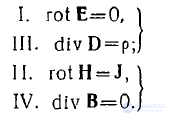
The first pair of equations involves quantities characterizing only the electric field. The second pair — quantities characterizing only the magnetic field. This means that at  electricity and magnetism — are distinct phenomena. The first pair of equations forms the basis of electrostatics; the second pair of equations is the initial system of equations of magnetostatics. To solve these pairs of equations, the corresponding constitutive equations must also be added. In this lecture we will begin studying electrostatics, which, accordingly, is defined by the equations
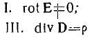
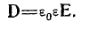
and in the simplest case of isotropic media by the constitutive equation
Equation 1 states that the electrostatic field is irrotational.
Since
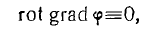
we can set,
 (1)
(1)

The scalar function is called the electrostatic potential or simply the potential.

Representing the electrostatic field by formula (1) means that this field is potential. The «—» sign is a matter of convention. It is placed so that <p has the meaning of potential
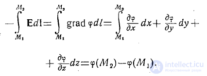
energy. More precisely, so that the work done by external forces (against the forces of the field) in moving a unit positive charge from one point of the field to another, for example from point M1 to point M2, equals the increase in the potential energy of this charge. According to (1) this work is equal to
 (2)
(2)
From formula (2) it follows that the work mentioned does not depend on the path along which the motion takes place, but depends only on the initial and final position of the charge. Consequently, when a charge is moved along a closed curve, the work will be equal to zero.
Formula (1) does not define the function φ completely, but only up to an arbitrary constant. However, in most cases one is interested in the potential difference, and the arbitrary constant
drops out. The arbitrary constant turns out to be equal to zero in the case where the electrostatic field under consideration is created by charges located in a bounded region of
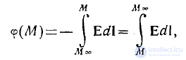
space. Then the potential at infinity is equal to zero, and at a point M located at a finite distance,
 (3)
(3)
where M∞ — is the point at infinity.
For a visual representation of the electrostatic field, as well as for calculations, the concepts of equipotential surfaces and field vector lines are introduced. Equipotential surfaces are defined by the equation

from which we obtain that on the equipotential surface

where d\ — is the element of line length on this same surface.
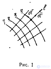
Consequently, the vector lines E are perpendicular to the equipotential surfaces. Let us find the equations of the vector lines E. Let dl' — be the element of line length (Fig. 1).
Since the vectors E and dl' are collinear, we have
that is 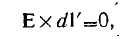
then 
from which we obtain
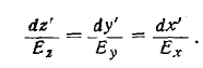
If Ex, Ey, Ez are known as functions of the coordinates x, y, z, then by solving this system of differential equations one can determine the desired vector lines E.
When classifying EM phenomena, it was noted that the electric field created by stationary electric charges is conventionally called electrostatic. In such a field there are no changes of charges and fields in time, so the time derivatives of all quantities are equal to zero ∂ ∂t = 0 , including j = −∂ρ ∂t = 0. The system of Maxwell's equations for this case splits into two independent pairs of equations, one of which describes the electrostatic field (2.21), and the other the magnetostatic field (2.22).
The third of Maxwell's equations in integral form can be used to find the electrostatic field created by symmetric uniformly charged bodies. However, the possibilities of this method are limited to a small range of simple problems, so in most cases Maxwell's equations in differential form are used to find electrostatic fields.
Let us transform these equations into a form convenient for solving. Consider some region of space V, consisting of two subregions V1 and V2, bounded by surfaces S1 and S2 (Fig. 6.1). We will assume that all the sources of the field – in this case electric charges with volume density ρ(x, y, z) – are concentrated in region V1, while region V2 is free of
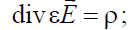
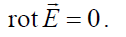
charges. The fields throughout the whole region V under consideration are described by the following Maxwell equations:
 (6.1)
(6.1)
 . (6.2)
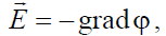
Let us analyze these equations. Equation (6.2) states that the sought electric field has no rotational components. Therefore, by virtue of (B.22) we can assume that the field intensity vector E
is the gradient of some auxiliary scalar function φ :
 (6.3)
(6.3)
which is called the electric scalar potential.
Substituting (6.3) into (6.1) we obtain an equation for the function φ:
 , (6.4)
which, under the assumption of homogeneity of the medium in both regions under consideration, transforms into the following form:
 , (6.5)
 . (6.6)
In writing equations (6.5) and (6.6) the symbolic Laplace operator (Laplacian) (B.17) was used. The first of these equations, called Poisson's equation, allows one to find the scalar electric potential in a region containing charges, while the second – Laplace's equation – is intended for finding the electrostatic field in a region free of charges.
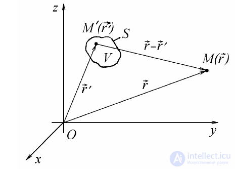
Figure 6.2
It can be shown that the solution of Poisson's equation for an unbounded region of space (Fig. 6.2) has the form
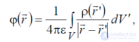
where rr and rr′ – are the position vectors of the observation point M and the source point M′ respectively; V – is the region where the charges are concentrated.
Let us now consider what physical meaning the electric scalar potential has. To do this, let us find the increment of the potential along the curve L (Fig. 6.2) when the point is displaced by a distance dl :

Now let us integrate the left and right sides of the obtained equation along L from point 1 to point 2:
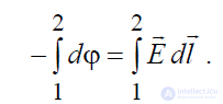
.
Since dφ is a total differential of the function φ , the integral on the left side of the equation does not depend on the path of integration and is determined by the value of the function at the endpoints.
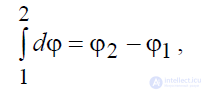 , (6.3)
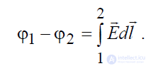
consequently, the potential difference at points 1 and 2 is determined by the expression:
 . (6.4)
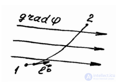
Figure 6.3
Comparing the obtained equality with expression (1.28), we conclude that the potential difference between points 1 and 2 is nothing other than the electric voltage between these points. Based on the physical meaning of voltage, we can conclude that the potential difference between points 1 and 2 – is the work done by electric forces in moving a unit charge from point 2 to point 1. A field possessing property (6.3) is conventionally called potential. Consequently, the electrostatic field is a potential field. The potential of a point at infinity is conventionally taken to be equal to zero,
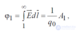
so, moving point 2 to ∞ , from (6.4) we can find the potential of the field at point 1:
 , (6.5)
from which it follows that the potential of the electric field at a given point is the work done by electric forces in moving to it from ∞ a unit charge q0 .
Let us dwell separately on the properties of conductors in an electrostatic field. Conductors are distinguished by the fact that they contain free electric charges, which under the action of the electric field are set in motion, that is, a conduction current with volume density j E
r r
σ = arises in them. Since in electrostatics it is conventional to take 0 ≡ j
r
, then for σ ≠ ∞ it is necessary to set E ≡ 0 , i.e. there is no electrostatic field inside conductors.
All free charges of a conducting body accumulate on its surface, where they take up an equilibrium position such that the fields they create inside the body mutually cancel. Since all electric charges are located on the surface of the conductor, in this case the surface charge density σs can be used to characterize the charged metallic body.
It is easy to show that the tangential component of the vector Er is absent on the surface of the conductor. Indeed, if it were not equal to zero 0 ≠ τ Er , then a surface current would exist, which is not allowed in electrostatics. It follows that all field lines of Er on the surface of the conductor are perpendicular to it. Since 0 = τ E r , all points of the surface have the same potential, i.e. the surfaces of a conductor are equipotential in electrostatics.
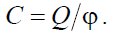
It is obvious that in order to bring different conductors to the same potential φ, a different amount of charge Q must be introduced onto them. From this
point of view, the concept of electric capacitance was introduced to characterize each conducting body, defined as
 (6.6)
(6.6)
By definition, electric capacitance – is the amount of charge that must be delivered to a conductor to charge it by one unit of potential.
In the SI system, capacitance is measured in Farads: C[Farad] = C V.
A system of two conductors is called a capacitor, and the capacitance of a capacitor is defined as
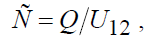 , (6.7)
where Q and U12 must have the same sign.
It is easy to show that the energy of a capacitor is equal to:
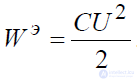 . (6.8)
The source of a stationary EMF is a conduction current constant in time , 0 ≠ j
r
where it is assumed that all sources and field vectors do not depend on time (∂ ∂t = 0 , except ∂ρ ∂t = C = const ). Maxwell's equations for this case have the form:
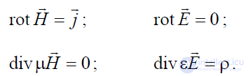
In this case the electric and magnetic fields are no longer independent, as in the case of static fields. The connection between them is provided by Ohm's law 
The equations for the stationary electric field coincide with the analogous equations for the case of electrostatics, so here too we can
use the concept of electric potential:
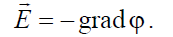
However, here 
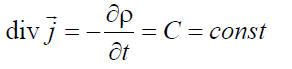
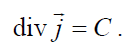
, so we cannot consider the electric field strength inside conductors to be equal to zero, nor the fields on the surface of conductors to be equipotential. To clarify the structure of the electric field inside a conducting medium, let us consider the continuity equation, which for this case has the form:
or
 (6.9)
(6.9)
Substituting here the current density from Ohm's law  , we obtain:
 (6.10)
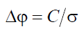
and for a homogeneous medium, where σ = Const :
 (6.11)
We have again arrived at the scalar Poisson equation for the scalar potential of the electric field in a conductor.
If there are no current sources in the region under consideration (  ), then this equation reduces to the Laplace equation:
Δφ = 0 , (6.12)
analogous to the case of static fields.
Thus, in media with finite conductivity, the equation obtained can be used to calculate the electric field strength and current density in the conductor.
Let us now consider the magnetic field excited by conduction currents.
From the first Maxwell equation one can find the magnetic field strength H
r
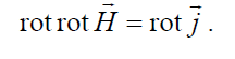
. To do this, let us apply the rot operation to both of its sides:
 (6.13)
Let us transform the left side of the obtained equation using identity (6.23):
 t (6.14)
which allows us to obtain the Poisson equation for the field strength Hr in vector form:
 (6.15)
It can be shown that the solution of this equation for unbounded space has the form:
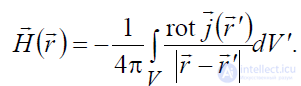 (6.16)
To obtain the presented solution of the vector Poisson equation, it is necessary to represent the vector Hr as an expansion over coordinate projections and thereby split the vector equation into three scalar ones. Then, applying known relations to solve the resulting scalar equations and combining them, one can obtain the desired formula (6.16). The presence of the differential operation j r
rot under the integral sign in formula (6.16) makes it difficult to apply for solving equation (6.15). Therefore, as in the case of electrostatics, to facilitate solving the problem, an auxiliary vector function Ar is introduced, which is called the vector magnetic potential:
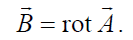 (6.17)
Substituting here H Br rμ= 1 into the 1st Maxwell equation, we have:
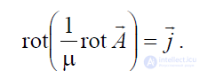 . (6.18)
If we assume that the medium in the region of space under consideration is homogeneous, i.e. μ = Const , then the last equation transforms into the form:

Let us transform the left side of the obtained equation using the vector identity (B.23), as a result of which we obtain:
 . (6.19)
The vector potential Ar introduced by this expression is defined up to the gradient of an arbitrary scalar function of the coordinates Ψ. Indeed, if to the introduced potential Ar
we add gradΨ, then the new potential A′ = A + gradΨr r will also satisfy equation (6.17), since rot gradΨ = 0 . To remove this ambiguity, let us assume that
0 div = Ar , then equation (6.19) takes the form:
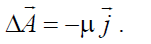 . (6.20)
Thus, in this case too we have obtained the vector Poisson equation, only now for the vector magnetic potential. This equation compares favorably with (6.15) in that its right side does not contain the differential operation rot. The solution of (6.20) can be written as:
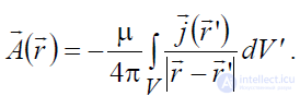 . (6.21)
In the region where 0 = jr
, the Poisson equation turns into the Laplace equation:
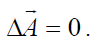 . (6.22).
Using the vector potential, it is quite simple to express another important parameter of the magnetic field – the magnetic flux:
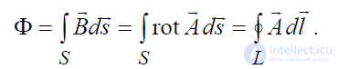 . (6.23)
It follows that the magnetic flux through the surface S is numerically equal to the circulation of the vector Ar around the contour L on which this surface rests. In deriving the last relation, Stokes' theorem was used to transform the surface integral into a contour integral. For conductors with a linear current, the ratio of the magnetic flux it creates to the current I is called the inductance:
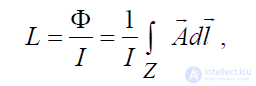
which does not depend on I and is a characteristic of the conductor itself.
Setting e = const and substituting 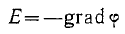 into equation I I I , we obtain
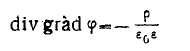
or
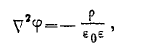 ( 4 )
( 4 )
where
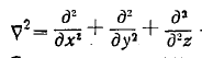 —the Laplace operator.
Relation (4) — is Poisson's equation; in those regions of space where there are no charges, i.e. p = 0, Poisson's equation turns into Laplace's equation
 (5)
(5)
Thus, the system of Maxwell's equations for the electrostatic field has been reduced to a single scalar Poisson or Laplace equation for the potential <p. Having found the potential, it is easy to calculate the field strength E from formula (1). Let us find the solution of equations (4) and (5). Let us begin with the simplest case — a point charge of magnitude g
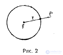
Such a charge creates a field whose vector lines E are directed along the radii. Owing to this spherical symmetry, the field E is determined very simply. For this, the third equation
of Maxwell in integral form is used
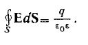
A sphere of radius r is drawn with its center at the point where the charge is located. Since the vector lines E are normal to this sphere, from the last relation we obtain
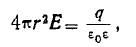
from which
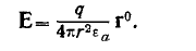
This field was found from the third Maxwell equation, and therefore it satisfies it.
The potential φ is found from formula (3):
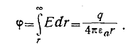
From this last formula it follows that since E =—gradcp.
the vector E thus found also satisfies the first Maxwell equation. Let us now consider a system of point charges q1, q2, q3, qn (Fig. 3).
Since Maxwell's equations are linear, using the superposition principle for the total potential of this system of charges
at a point with coordinates — x, y, z (the observation point), we can write
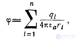
where

This result can be generalized to the case of a continuous charge distribution and written (Fig. 4)
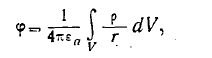 (6)
(6)
where

Formula (6) is obviously a solution of Laplace's equation (5), since it is a generalization of the formula for a discrete system of point charges, in which the potential was determined
not at these points.
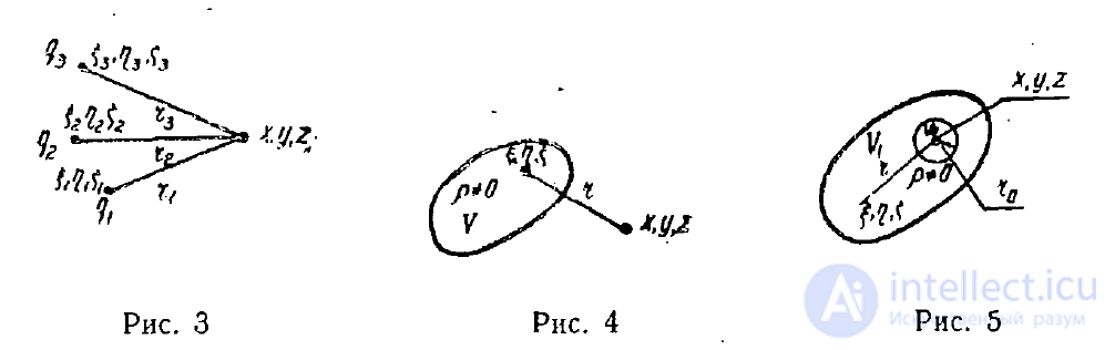
However, we will now show that formula (6) is also a solution of Poisson's equation. Indeed, let the observation point with coordinates x, y, z be located in the region where 
(Fig. 5). Then, by isolating this point, surrounding it with a sphere of small radius  o and volume Vo, we can write for the potential created by the charges
in the rest of the volume V
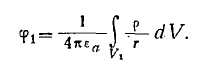
Let us examine the expression
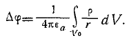
Obviously,

Thus it is proved that for Poisson's equation too the solution
is the expression
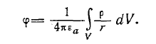
Poisson's equation (or the inhomogeneous Laplace equation) can in general be written in the following form:
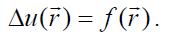 . (6.24)
In the case f (r ) = 0 r this equation becomes homogeneous and is called Laplace's equation:
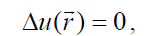 , (6.25)
where f (r ) r – is a given function of the coordinates, u(r ) r – is the unknown function of the coordinates, ( rr – the position vector of a point in space) r ∈V r , V – is a given region
of space in which u(x, y, z) must be found.
It has been proved in mathematical physics that the problem has a solution if boundary (or edge) conditions are given on the boundary S bounding the region V under consideration. Three types of boundary conditions are distinguished:
1) Dirichlet boundary conditions, when the value of the sought function is known on the boundary of the region:
 (6.26)
2) Neumann boundary conditions, when the value of the normal derivative of the sought function is given on the boundary of the region:
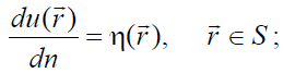 (6.27)
3) mixed boundary conditions (generalized Neumann boundary conditions), when both Neumann and Dirichlet conditions hold simultaneously on the surface S:
 , (6.28)
where q(r) r and p(r ) r – are known functions. In the case q(r ) = 0 r these conditions reduce to Neumann conditions, and in the case q(r )→∞ r they turn into Dirichlet conditions.
Depending on the type of boundary conditions used, the problem of finding u(r ) r from Poisson's equation (6.24) is called, respectively, the Dirichlet boundary-value problem, the Neumann boundary-value problem, or the mixed boundary-value problem.
Analytical or numerical methods are used to solve the boundary-value problem.
Analytical methods make it possible to obtain an exact solution of the boundary-value problem. The most commonly used of them are:
1) the method of separation of variables (Fourier method);
2) the method of conformal transformations;
3) the method of Green's functions.
A general drawback of analytical methods – is the very limited range of problems to which these methods are applicable. Mainly, these are problems of determining fields in regions of space whose boundaries coincide with coordinate planes in one of the known coordinate systems.
Numerical methods belong to the approximate methods of solving equations. The most frequently used are:
1. The finite-difference method (grid method)
2. The finite element method.
The main advantage of numerical methods is that they have practically no restrictions on the geometry of the problem, while their main drawback – is that they do not make it possible to obtain an exact solution.
Let us consider two of the most commonly used methods for solving Poisson's equation, one of which belongs to the group of analytical methods, and the second – to numerical ones.
According to the above, we can write
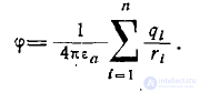
The position of the observation point will be characterized by the position vector r, and the position of the charges will be characterized by the vector
/,: (Fig. 6), where we will assume that

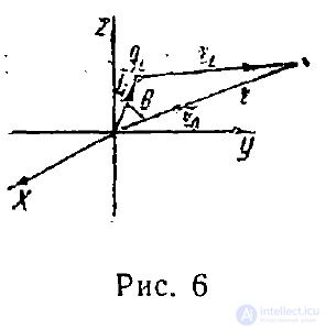
Then we can assume
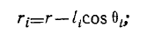

and, consequently,

since
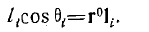
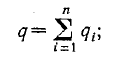
From this expression (7) two important conclusions can be drawn:
1) at large distances from the system, the potential is the same as the potential of a single point charge of magnitude
2) if the system is neutral, i.e.
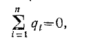
then the potential is inversely proportional to the square of the distance and equal to
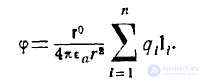
The vector  / is called the electric moment of the system of charges. A property of this vector — its magnitude does not depend on the origin. Indeed, let the origin be shifted by
a
and let і! be located at point O' (Fig. 7). Then
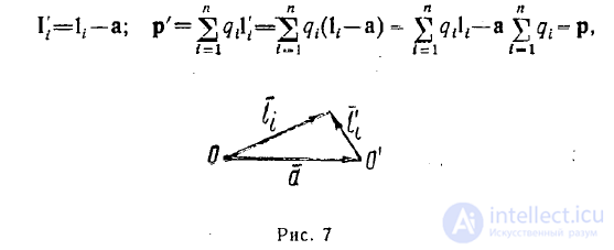
i.e. the moment is the same as if there had been no shift of the origin
Let us obtain the solution of Poisson's equation in general form, using the method of Green's functions. For this, consider some region of space V (Fig. 6.4), in which we isolate two subregions V1 and V2 (V = V1 ∪V2 ). Let the field sources with given distributions of charge densities (r ') r ρ or current densities j(r ') r r be concentrated in one of the subregions (V1)
, rr′∈V1, while
the second subregion (V2 ) is free of field sources (charges and currents).
Let boundary conditions (Dirichlet, Neumann, or mixed) be given on the surface S2 bounding the volume V.
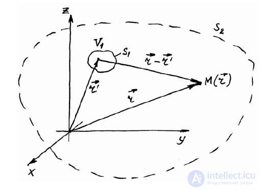
Figure 6.4
The field throughout the whole region under consideration is created by sources concentrated in subregion V1, so any point M′(r ′) r
here is conventionally called the source point, and the position vector indicating its location in the chosen coordinate system is usually called the position vector of the source point. The point M(r ) r , where the electromagnetic field is observed, is called the observation point, and r ∈V r – is the position vector of the observation point.
Let us introduce the auxiliary function G(r, r ') r r , which is called the Green's function and is a solution of Poisson's equation for the region V under consideration, whose right-hand side is the Dirac δ-function:
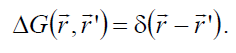 . (6.29)
The δ-function used in (6.29) belongs to the class of generalized functions and possesses the following properties:
1) the δ-function is equal to zero throughout the whole region, except at the point r = r ′ r r :

2) at the point r = r ′ r r the δ-function tends to infinity:

3) the convolution of the function (r r ') r r δ − and any other function f (rr′) defined in V is equal to the value of the latter at the point rr :
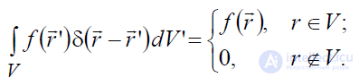 (6.30)
Expression (6.30) is usually taken as the definition of the Dirac δ-function. In particular, if f (r ′) = 1 r , it transforms into the form:
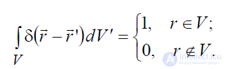 (6.31)
For three-dimensional unbounded space, the δ-function can be represented as
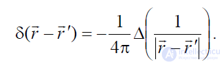 . (6.32)
Let us find the solution of Poisson's equation (6.24), for which we use the second Green formula (B.28):

Assuming here that u(r ) r φ = – is the sought function, and Ψ = G(r − r ′) r r – is the Green's
function, we have:

.
Substituting into the left side of the last equation Δu(rr) from (6.24) and ΔG(r − r ′) r r from (6.29), it is easy to arrive at the equality:

Using the basic property of the δ-function (6.28) we finally find:
 (6.33)
We have obtained the solution of Poisson's equation in explicit form, where the sought
function u(r ) r is expressed in terms of the known excitation function f (r ) r and the Dirichlet and Neumann boundary conditions, which are given by the conditions of the problem. In the case where f (r ) = 0 r , the first integral on the right side vanishes, and then (6.33) represents the solution of Laplace's equation. In this case the sought function is determined only by the boundary conditions given on the surface S.
Two important remarks must be made regarding the solution obtained:
1) to find u(r ) r from expression (6.33) it is necessary that both the value of the function and its derivative be given simultaneously on the boundary S;
however, it can be proved that the last two integrals on the right side of (6.33) are interrelated, and therefore, for a unique solution of the
Laplace and Poisson equations it is sufficient to know one of the Dirichlet or Neumann boundary conditions∗;
∗ The solution of the interior Neumann problem is determined up to an additive constant.
2) to use expression (6.33) it is necessary to know the Green's function for the region under consideration, which would satisfy equation (6.29) and the given boundary conditions.
Let us find the solution of Poisson's equation for unbounded space. In this case the surface S must be moved to infinity. Assuming
that the fields at infinity decrease no slower than 1/ r , it is easy to establish that both surface integrals on the right side of (10) vanish, and this expression itself takes the form:
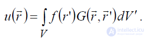 (6.34)
Comparing equations (6.29) and (6.32) with each other, it is easy to arrive at the conclusion that the Green's function of Poisson's equation for free space
can be represented as:
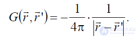
Substituting the found Green's function into (6.34), we find the solution of Poisson's equation for free space:
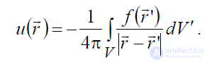 . (6.35)
Now, using expressions (6.24) and (6.35), it is easy to find the solution of the vector Poisson equation
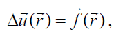 , (6.36)
by splitting it into three scalar ones, which in the case of unbounded space gives:
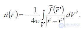 (6.37)
In particular, using expressions (6.35) and (6.36), to determine the scalar (r ) r φ and vector A(r ) r r potentials of the electric and magnetic fields created respectively by electric charges and currents, the following formulas can be obtained:
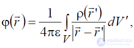 , (6.38)
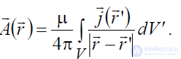 . (6.39)
Based on expressions (6.33) and (6.35)-(6.37), it can be said that the method of Green's functions makes it possible to obtain an integral representation of the exact solution of the scalar and vector Poisson and Laplace equations, but requires determining the Green's function for the given region of space, which is not always simple to do by analytical methods.

Comments