2.8. Classification of Electromagnetic Phenomena and Fields — Static, Stationary, Quasi-static, Non-stationary

Lecture

The classification of electromagnetic phenomena in the theory of the electromagnetic field is based on various manifestations of the interaction of electric and magnetic fields, their sources, and their properties.

Based on the dependence of the field characteristics on time, a classification of electromagnetic phenomena is introduced.
1. Static field 2.8. Classification of Electromagnetic Phenomena and Fields — Static, Stationary, Quasi-static, Non-stationary . Fields unchanging in time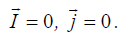

.
The system of Maxwell's equations splits into two independent systems, one of which describes the fields of stationary charges (electrostatics):
, (2.20)
and the second – the fields of permanent magnets (magnetostatics):
2.8. Classification of Electromagnetic Phenomena and Fields — Static, Stationary, Quasi-static, Non-stationary . (2.21)
2. Stationary EMF – this is the field created by direct (constant) currents:

2.8. Classification of Electromagnetic Phenomena and Fields — Static, Stationary, Quasi-static, Non-stationary . (2.22)
3. A quasi-static field is created by slowly varying currents, when it can be assumed that
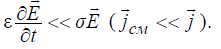. (2.23)
4. Non-stationary (rapidly varying) field – is described by the full system of Maxwell's equations.

Electromagnetic phenomena cover a wide range of physical processes, from static fields to high-energy electromagnetic waves. These phenomena are unified by Maxwell's equations, which serve as the fundamental basis of the theory of the electromagnetic field. The classification simplifies their study and helps to understand the regularities of the interactions.

Unlike the electrostatic field, a stationary electric field exists not only in a dielectric, but also in a conductor in the presence of a constant conduction current. The equations of the stationary electric field are similar to the equations of the electrostatic field (σ =const):

2.8. Classification of Electromagnetic Phenomena and Fields — Static, Stationary, Quasi-static, Non-stationary (12.16)

The potential of the stationary field is determined by Poisson's equation (11.11). 2.8. Classification of Electromagnetic Phenomena and Fields — Static, Stationary, Quasi-static, Non-stationary

The volume charge density is expressed by the formula:

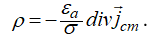2.8. Classification of Electromagnetic Phenomena and Fields — Static, Stationary, Quasi-static, Non-stationary . (12.17)

From (12.16) it follows that volume electric charges can exist only in those regions of a conducting medium where extraneous currents are absent.

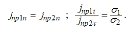At the interface between two conducting media, the current lines are refracted in accordance with the boundary condition (4.3) 2.8. Classification of Electromagnetic Phenomena and Fields — Static, Stationary, Quasi-static, Non-stationary :

2.8. Classification of Electromagnetic Phenomena and Fields — Static, Stationary, Quasi-static, Non-stationary . (12.18)

If the conductivities of the media differ strongly (σ2>>σ1), then in the weakly conducting medium 2.8. Classification of Electromagnetic Phenomena and Fields — Static, Stationary, Quasi-static, Non-stationary passes practically along the normal, regardless of the orientation of the current density vector in the medium with the higher conductivity. In this case, the surface of metallic bodies located in a dielectric can be considered equipotential (σ=const).

In some cases, for a stationary electric field in a region free of extraneous charges and currents, the method of electrostatic analogy is applicable, which allows the problem of the stationary electric field to be reduced to problems of electrostatics. In this case, the boundary conditions for the components of the current density vector are analogous to the boundary conditions for the electric displacement vector. The transition to the equations of electrostatics for systems with identical geometric dimensions is carried out using the following change of variables:

2.8. Classification of Electromagnetic Phenomena and Fields — Static, Stationary, Quasi-static, Non-stationary (12.19)

The method of electrostatic analogy is used in the analysis of the EMF of transmission lines with a T-wave (coaxial line, etc.). On the other hand, the electrostatic analogy allows complex electrostatic fields to be studied experimentally by modeling them in a tank with a weakly conducting liquid (electrolyte).

The equations of the stationary magnetic field are written in the form:

2.8. Classification of Electromagnetic Phenomena and Fields — Static, Stationary, Quasi-static, Non-stationary . (12.20)

In (12.20) a connection between the electric and magnetic fields is already noticeable.

The most common problem is determining the stationary magnetic field for a given current distribution. For an isotropic, linear, homogeneous medium, it is convenient to analyze the EMF using 2.8. Classification of Electromagnetic Phenomena and Fields — Static, Stationary, Quasi-static, Non-stationary .

2.8. Classification of Electromagnetic Phenomena and Fields — Static, Stationary, Quasi-static, Non-stationary

For the vector potential of the stationary magnetic field, the gauge condition (11.6) and the wave equation (11.7) are written in the form:

, 2.8. Classification of Electromagnetic Phenomena and Fields — Static, Stationary, Quasi-static, Non-stationary . (12.21)

The solution of (12.21) with respect to A(r) corresponds to the solution of the Helmholtz wave equation at k=0 :

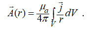2.8. Classification of Electromagnetic Phenomena and Fields — Static, Stationary, Quasi-static, Non-stationary . (12.22)

In simple cases, in the presence of field symmetry, it may be more convenient to directly calculate 2.8. Classification of Electromagnetic Phenomena and Fields — Static, Stationary, Quasi-static, Non-stationary using (3.4).

For example, due to cylindrical symmetry, it is convenient to find the magnetic field of a round wire with current and of a coaxial line precisely using (3.4).

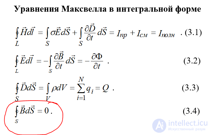
2.8. Classification of Electromagnetic Phenomena and Fields — Static, Stationary, Quasi-static, Non-stationary

The integration contour is conveniently combined with the vector field lines 2.8. Classification of Electromagnetic Phenomena and Fields — Static, Stationary, Quasi-static, Non-stationary .

For a round wire of radius a with electric current I:

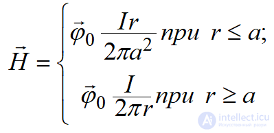2.8. Classification of Electromagnetic Phenomena and Fields — Static, Stationary, Quasi-static, Non-stationary . (12.23)

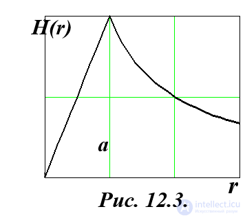
A graph of the magnetic field distribution in the conductor H(r) is shown in fig. 12.3.

2.8. Classification of Electromagnetic Phenomena and Fields — Static, Stationary, Quasi-static, Non-stationary

For a coaxial transmission line (fig. 12.2):

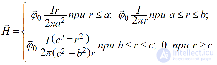2.8. Classification of Electromagnetic Phenomena and Fields — Static, Stationary, Quasi-static, Non-stationary . (12.24)

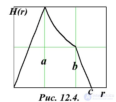
A graph of the magnetic field distribution in the coaxial line is shown in fig. 12.4.

The derivation of these formulas, as well as other examples of stationary magnetic fields, can be found in [Falkovsky O. I. Technical Electrodynamics: Textbook for Communications Universities. - M.: Svyaz, 1978. - 432 p.].

Energy of the stationary magnetic field:

2.8. Classification of Electromagnetic Phenomena and Fields — Static, Stationary, Quasi-static, Non-stationary . (12.25)

Comparing with (12.6), one can notice a certain similarity between the equations of the stationary magnetic field and the equations of electrostatics.

The total energy of the stationary magnetic field of a system of n circuits with currents is conveniently expressed through the currents and inductances (see the explanation for (9.18)):

2.8. Classification of Electromagnetic Phenomena and Fields — Static, Stationary, Quasi-static, Non-stationary , (12.26)

where 2.8. Classification of Electromagnetic Phenomena and Fields — Static, Stationary, Quasi-static, Non-stationary – is the flux linkage of the k-th circuit, – is the self-inductance of the k-th circuit, – is the mutual inductance of the j-th and k-th circuits.

The first term of (12.26) represents the sum of the self-energies of the magnetic fields of the circuits, while the second term of (12.26) – represents the mutual energy of the magnetic fields created by the currents in these circuits.

By analyzing the stored magnetic energy in the system, one can calculate the inductance of conductors and T-wave transmission lines.

The magnetic flux passing through the cross section of a transmission line is conveniently decomposed into internal and external components. The internal flux, passing inside the conductors, is associated with the self-inductances of the conductors.

The external magnetic flux is determined by the field lines 2.8. Classification of Electromagnetic Phenomena and Fields — Static, Stationary, Quasi-static, Non-stationary in the medium external to the conductors, and is associated with the mutual inductance.

For example, the inductance per unit length of a coaxial transmission line (fig. 12.2) under direct current is determined by the formula ( μ 1 – μ of the dielectric, and μ 2 – μ of the conductors):

2.8. Classification of Electromagnetic Phenomena and Fields — Static, Stationary, Quasi-static, Non-stationary . (12.27)

The first term of (12.27) corresponds to the mutual inductance of the conductors, and the second – to the self-inductance. Reference books usually give formula (12.28), which corresponds to a high-frequency current:

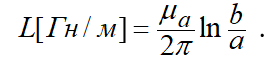2.8. Classification of Electromagnetic Phenomena and Fields — Static, Stationary, Quasi-static, Non-stationary . (12.28)

it should be remembered that in this formula a – is the absolute magnetic permeability of the dielectric.

The inductance of a two-wire transmission line (fig. 12.1) (1 – of the dielectric, and 2 – of the conductors) is calculated in a similar way:

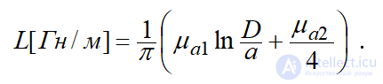2.8. Classification of Electromagnetic Phenomena and Fields — Static, Stationary, Quasi-static, Non-stationary . (12.29)

The first term of (12.29) corresponds to the mutual inductance of the conductors, and the second – to the self-inductance of the two cylindrical conductors. Reference books usually give formula (12.30), which corresponds to a high-frequency alternating current [4, 5, 11]:

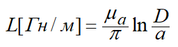2.8. Classification of Electromagnetic Phenomena and Fields — Static, Stationary, Quasi-static, Non-stationary . (12.30)

When analyzing multiconductor T-wave transmission lines (in which the number of conductors is greater than two) and connections using them, matrices of mutual capacitances and inductances of the line conductors are compiled based on (12.6) and (12.26).

A quasi-stationary EMF in a region V is one for which the wave character can be neglected. For a quasi-stationary field, the time during which the field sources manage to change noticeably is large compared to the delay time of the wave front (l/v). (l – is the distance in the region V, which the propagating EMW traverses at speed v.)

The delay time – is the time required for the EM disturbance to propagate from one end of the system to the other.

The following relations hold for a quasi-stationary EMF:

2.8. Classification of Electromagnetic Phenomena and Fields — Static, Stationary, Quasi-static, Non-stationary , . (12.31)

In the case of monochromatic oscillations, the plane wave turns into an oscillation in time: 2.8. Classification of Electromagnetic Phenomena and Fields — Static, Stationary, Quasi-static, Non-stationary , from which follows another condition for the quasi-stationarity of the field:

Thus, for monochromatic processes, EM systems can be studied using the laws of the quasi-stationary EMF in those cases when their extent is much smaller than the wavelength.

A rapidly varying EMF is described by the full system of Maxwell's equations without any simplifications, is characterized by a deep interconnection between electric and magnetic phenomena, and has a wave character.