
Lecture
The methods for solving Maxwell's equations and the properties of the resulting solutions depend substantially on the shape of the region of space in which the EMF is defined, the electrophysical properties of the medium filling it, the distribution of excitation sources, and the given boundary conditions. In this regard, the problems of finding electromagnetic fields can be divided into two groups: internal and external problems of electrodynamics.
An internal problem is the problem of finding the electromagnetic field in a finite volume V, which is bounded on all sides by a closed surface S. In other words, as a result of solving the internal problem we find the electromagnetic field inside some closed volume V.
The external problem of electrodynamics consists in finding the fields in unbounded space, except for certain regions in which this
field may be absent. In this case we find the fields outside some volume V, and therefore the problem is called external.
Let us consider the conditions for the existence and uniqueness of both of these problems of electrodynamics.
Consider a region of space V, filled with
a linear medium with known parameters, in which there are sources of the electromagnetic field j
r
.
It is known that the field inside the selected region can be described by a system of Maxwell's equations. Let us prove that the solution of this system for given boundary conditions and a known distribution of field sources will be unique. To do this, let us formulate the uniqueness conditions for the solution of internal problems of electrodynamics in the form of the following theorem.

The internal problem of electrodynamics will have a unique solution
if any of the following boundary conditions is specified on the surface S bounding the region of space under consideration:
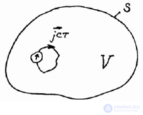
Figure 5.1
We shall prove the theorem by contradiction, i.e. suppose that as a result of solving the stated problem
two different solutions could be obtained: one of which is a field described by the vectors 1 E&r
, and the second – by the vectors 
. Both of these solutions must satisfy Maxwell's equations, so we can write:

Subtracting the second pair of equations from the first pair, we obtain:

The field difference 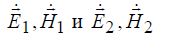

represents a third field 
. If we prove that this field is identically equal to zero, this will mean that there is no difference between the assumed solutions, i.e. the system of Maxwell's equations has a unique solution.
is a linear combination of the solutions, which must satisfy the following system of equations:
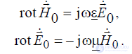
Applying the Umov–Poynting theorem for the field  in the volume V under consideration and retaining in it only the equality of the real terms, we can obtain the following relation:
 , (5.3)
where it is taken into account that 
Let us transform the integrand on the left-hand side of the last equality, using the property of the scalar triple product of three vectors:

It follows that the integrand on the left-hand side of equality (5.3) is proportional to the tangential components of the electric or magnetic fields
– τ 0 E& r
or τ 0 H&
on S. However, by virtue of the boundary conditions (5.1) specified on S, which both solutions of the problem must obey, one of the following two equalities holds:

which, together with equalities (5.2), leads to the following identities:

Consequently, the integral on the left-hand side of the equality under consideration is equal to zero:
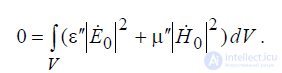 . (5.4)
Let us now consider the integral on the right-hand side of (5.4). Suppose that the imaginary
parts of the permittivity and permeability of the medium inside the volume V
are not equal to zero ( ε′′ ≠ 0 and μ′′ ≠ 0). This can occur in two cases:
a) when energy absorption takes place in the medium, then ε′′ > 0, μ′′ > 0 ;
b) the medium is regenerative (i.e. it is itself a source of energy), then ε′′ < 0 , μ′′ < 0.
In the general case, the right-hand side of equality (5.4) will equal zero only when
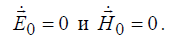
. (5.5)
These last equalities are the proof of the uniqueness theorem for the solution of internal problems of electrodynamics.
Thus, we have proved that the solution of the internal problem of electrodynamics exists and is unique if
a) the medium filling the volume V is absorbing or regenerative;
b) the tangential component of the electric τ Er or magnetic τ Hr field is specified on the surface S.
Let us pose the problem as follows. Suppose that in the region of space under consideration there is some bounded volume V1, in which all field sources are concentrated.
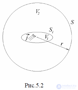
These sources create an electromagnetic field in the surrounding space, including
the space external with respect to volume V1.
This field can be found by solving
the system of Maxwell's equations. Let us find the conditions under which the solution of this system
is unique for the region of space external with respect to the volume
V1. Let us surround this volume with a sphere of large radius r and seek the solution
of the problem inside this sphere, in the volume V2, enclosed between the surfaces
S1 and S2, where there are no field sources.
In this case we are dealing with the internal problem of electrodynamics, whose uniqueness we have proved above. For this it is necessary that
the medium inside V2 be absorbing or regenerative ( ε′′ ≠ 0, μ′′ ≠ 0), and also that there be no flux of the Poynting vector of the difference field 0 0,H E & r
& r
through
the surface bounding it. In this case the last condition has the form:
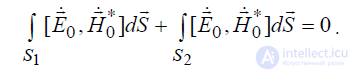 . (5.6)
Let the boundary conditions (5.1) be specified on S1, from which it follows:

then
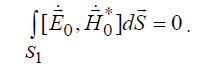
.
To prove the theorem we need to find the conditions under which
the second integral in (5.5) vanishes.
Let us begin to increase the radius of the sphere we outlined without bound, i.e. let r → ∞. In a spherical coordinate system the differential dS = r 2 sin θ dθ dϕ, so it is easy to establish that in order for
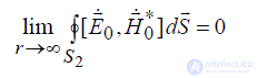
it is necessary that the amplitudes of the field strengths 0 0,H E & r
& r
as r → ∞
decrease faster than
r
1 . Then

Thus, the uniqueness conditions for the solution of the external problem of ED
can be formulated as follows:
The solution of the external problem of ED exists and is unique if
a) the medium filling the space is absorbing;
b) on the surface S1 of the region V1, outside of which the field is determined, the
tangential components Eτ or Hτ are specified;
c) the amplitudes of the electric and magnetic field strengths E& and
H& as r →∞ decrease faster than 1 r (the Sommerfeld condition).
5.4. The Principle of Permutational Duality of Maxwell's Equations
We already know that the EMF in space is excited by electric
charges and currents. The distribution of these currents and charges is in most cases quite complex, which noticeably complicates the solution of the problem
of determining the fields. In such cases various techniques are adopted to
somehow facilitate its solution. One such technique, which in a number of
cases can substantially help in solving Maxwell's equations, consists in
introducing fictitious magnetic currents and charges.
The possibility of introducing them stems from the fact that with them we replace perfectly
definite electric currents and charges, on the condition that the magnetic sources create in the surrounding space the same EMF as the real
electric sources. In other words, to facilitate the solution of Maxwell's equations, we replace a given set of currents and charges, which are the real sources of the field, with another set of field sources – fictitious magnetic charges and currents, which create
the same EMF as the real sources. The magnetic sources are considered fictitious because in reality they do not exist in nature, and their introduction is a certain mathematical technique that facilitates the solution of a
particular problem. So, if in the original system of Maxwell's equations the real electric field sources are replaced with their equivalent fictitious magnetic field sources (i.e. the substitutions j& r
for jm& r
and ρ& for
ρ&m are made in them), we obtain a new system (see Table 5.1).
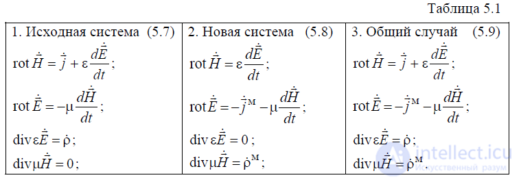
Here dt d j m m div ρ − = & & r
It is easy to see that the system of equations (5.8) can be obtained from (5.7) and
vice versa, if the following substitutions are made in them:
 . (5.10)
Combining expressions (5.7) and (5.8) makes it possible to obtain the generalized system of Maxwell's equations (5.9), which contains both electric and magnetic field sources. It is easy to show that the generalized system (5.9) remains unchanged when the permutations (5.10) are performed. This property is called the permutational duality
of Maxwell's equations.
How can this property be used?
Suppose that we know the solution of problem No. 1 of finding the fields
E& r
and H& r
in a given region V, created by a known distribution of electric field sources ρ& and j& r
. Suppose now that it becomes necessary to solve another problem (No. 2), which differs from the previous one
only in that the sources of the field in it are magnetic currents and charges m j& v
and ρ& , distributed in space exactly as the electric ones were in the previous problem. In this case there is no need for a detailed solution of problem No. 2, since it can be obtained directly from the solution of problem
No. 1, using the property of permutational duality of Maxwell's equations. To do this, in the expressions already found for the fields E& r
and H& r
as a result of solving problem No. 1, the substitutions (5.10) must be made, and we obtain the ready-made solution of problem No. 2. The solution found in this way satisfies
the new boundary conditions on the surface S, obtained from the previous ones by the same substitutions. If, for example, in the original problem
the tangential component of the field H
r
on S was equal to zero, then now the tangential component of the field E
r
must vanish.
Thus, the principle of permutational duality of Maxwell's
equations makes it possible to substantially facilitate the solution of many important practical problems of electrodynamics, and, therefore, has found wide application in
the theory of the EMF.
Let us obtain a certain auxiliary mathematical relation, called the Lorentz lemma, which is of particular importance in the formulation and solution of boundary-value problems of electrodynamics. To do this, consider an unbounded
isotropic medium with parameters
ε, μ, σ, σm, in which are compactly located
two regions of space V1 and V2, each of which has its own sources
of an electromagnetic field of a single frequency.
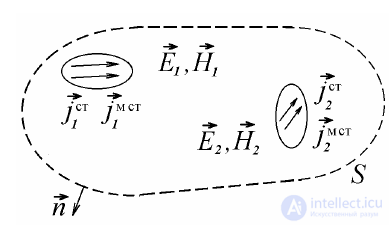
Figure 5.3
Let these sources be given by distributions of volume electric and
magnetic currents 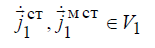 and
and 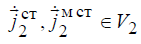
. Then the currents  create an electromagnetic field in the surrounding space
 , and the currents
 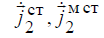 – the field
. Each of these fields is related to the currents exciting it by its own system of Maxwell's equations.
Let us write these two systems and then multiply the left- and right-hand sides of the equations scalarly by the vectors 
, as shown in the following formulas:

As a result of the multiplication we have:

Subtracting the lower equalities from the upper ones, we obtain:

Let us now add the resulting equalities and use the identity known from vector
analysis (B.19):

as a result of which we obtain an equality that has been named the Lorentz
lemma in differential form

Let us surround both regions of space under consideration with a single surface
S (fig.5.3) and integrate the left- and right-hand sides of the resulting equality
over the volume V bounded by this surface:
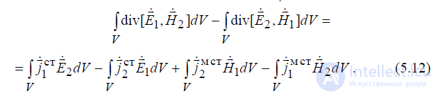
Applying the Ostrogradsky–Gauss theorem to the left-hand side of equality (5.12),
we obtain the Lorentz lemma in integral form, which
has the following form:

Relations (5.11) and (5.13) are quite frequently used in the theory
of the EMF, in particular when constructing integral equations for determining the distribution of electric currents induced by an electromagnetic field on conducting bodies, and also for proving certain theorems.
Below, using the Lorentz lemma, we shall prove the reciprocity theorem, which
is important for the theory of the EMF, especially when solving problems of radiation and scattering of electromagnetic waves.
Consider an infinitely extended isotropic medium with arbitrary parameters ε,μ, σ.
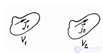
Figure 5.4
Let us specify in some volume V1 a distribution of currents 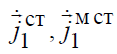
, and in volume V2 – 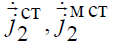
and apply the Lorentz lemma to this electromagnetic system.
To do this, let us surround both volumes with the surface
of a sphere S and let its radius r → ∞.
From the radiation condition at ∞ the surface integral in (5.13) tends to
zero and from the lemma there remains the equality:
 , (5.14)
which represents the mathematical formulation of the reciprocity theorem (or principle).
Let us explain this principle with a concrete example. Let V1 and V2 be thin conductors of radius a with axial currents  and
and 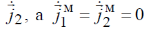
(fig.5.5). Assume that the distance between the wires is significantly greater than their lengths:
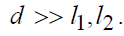
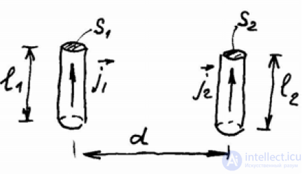
Figure 5.5
Then the remaining integral on the left-hand side can be written as

where I1 – the current flowing in the 1st wire; E21 – the EMF induced in the first wire by the field created by the current in the second wire.
Similarly, we transform the remaining integral on the right-hand side:

where I2 – the current flowing in the 2nd wire; E21 – the EMF induced in the 1st wire by the field created by the current in the 2nd wire.
Substituting the found values of the integrals into (5.14), we arrive at the relation:
 . (5.15)
At I1 = I2 → E12 = E21.
Thus, if the medium is isotropic, then the current I2 flowing in the 2nd wire induces in the 1st wire the same EMF as the current I1, flowing in the first wire, induces in the 2nd wire. This principle is fundamental in antenna theory. In particular, it follows from it that the parameters of antennas in receiving mode coincide with the analogous parameters of antennas in transmitting mode.
Consider infinite space in which the field sources 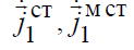 are compactly concentrated.
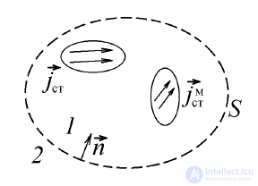
Figure 5.6
To determine the field created by these sources in the external space, it is necessary to solve Maxwell's equations for the unknown vectors E& r and H& r
. For a unique solution of this problem, in addition to the distribution of sources in space, it is also necessary to know the boundary conditions for the tangential components of the electric or magnetic field at the boundaries of the region under consideration (if they exist). At the same time, in practice situations often arise in which it is difficult to specify the exact spatial distribution of the real extraneous field sources, but it is possible to describe the field that they create on some imaginary closed surface S surrounding these real sources (fig.5.6). Let us denote the internal region of space with field sources (fig.5.6) with index 1, and the external one – with index 2. Since the surface S is imaginary, the field of the extraneous sources passes freely from 1 to 2. At the same time, we can formally write the boundary conditions for the tangential field components on this surface.
For the tangential component of the magnetic field, the boundary condition for the magnetic field strength on the surface S, taking into account the direction of the normal vector n (fig.5.6), will have the form:
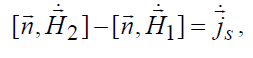
where  – the surface density of electric current on S.
Let us rewrite this equality in the form:
 , (5.16)
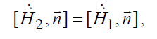
In our case the chosen surface is imaginary, i.e. it does not actually exist, so 0 = sj r
and the last equality takes the form:
 , (5.17)
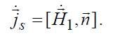
On the other hand, the field in region 2 would not change if we replaced the imaginary surface S with a real one that is also perfectly conducting, on which we would assume the existence of a surface current density found from the relation:
 . (5.18)
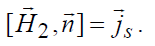
Then in equality (5.17) we must make the corresponding substitution, as a result of which it transforms to the form:
 (5.19)
Conditions (5.17) and (5.19) are equivalent by virtue of (5.18), so from a formal point of view it does not matter which of these boundary conditions is taken into account when solving the stated problem.
If we choose the latter condition, it turns out that we must formulate the problem of determining the field in the external region as follows.
Let us use the rule of permutational duality:

from which we obtain the boundary condition for the case of the existence of magnetic currents on the surface S:
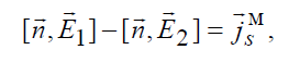
In the case under consideration our S is imaginary, so there are no currents on the surface at all. However, from a formal mathematical point of view, for determining the field in region 2 it makes no difference to us whether we know the field  on S, or the currents – the problem will have a unique solution.
In fact:

On the other hand we can denote: 
and consider this problem in the following formulation: determine the field in
the external region 2, if the field in region 1 is absent ( 1 Er, 0 1 = Hr), and on the surface S there exist equivalent currents 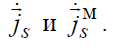 .
.
The boundary conditions in this case remain in the form 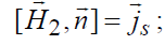
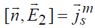
the solution of the problem outside the volume V will be the same as in the previous case. Thus, we have gone from the problem of determining the field outside
the volume V from the known distribution of sources in region 1 to the equivalent problem of determining the same field from the known distribution of surface currents on the surface S. Since we are dealing with only one field, the indices 2 can be dropped and we can write the expression for the equivalent currents:
 . (5.20)
Now we can formulate the equivalence theorem:
The field in a region of space free of sources will not change if the real sources are replaced by equivalent surface currents
on the boundary of the region, and all fields outside this region are set equal to zero.
We have formulated the above theorem on the basis of simple logical reasoning. This theorem can be proved rigorously using the Lorentz lemma.
Here we shall obtain two more useful mathematical transformations, known as Green's theorems (or formulas), and extremely useful
in various kinds of studies. These transformations follow directly from the Ostrogradsky–Gauss theorem:

Let us introduce two scalar functions φ and ψ, continuous in V together with their derivatives. Using them, we form the following two vectors:  . Substituting one of these vectors, for example 1 A
r
, into formula (5.21) in place of the vector Ar, we obtain the expression:

Let us transform the integrand on the left-hand side of the resulting equality, using the identity known from vector analysis (B.19):

Now let us consider the integrand on the right-hand side of equality
(5.21):

,
where gradn ψ – the projection of the gradient onto the normal, numerically equal to the derivative of the function 
along the direction of the normal to the surface S.
Taking into account the transformations made, it is easy to obtain the following relation:

which represents Green's theorem in its 1st formulation (or the 1st Green's formula).
Now let us return to relation (5.21) and substitute into it the vector 2 Ar in place of the vector Ar, and then perform on it the same operations that were performed on the vector 1 A
r
, as a result of which we arrive at the following relation:

Subtracting equality (2.23) from equality (5.24), we obtain Green's theorem in its 2nd formulation (or the 2nd Green's formula):

Both of Green's formulas are very often used to prove many fundamental propositions of electrodynamics, and also to obtain solutions of boundary-value problems of electrodynamics formulated in the form of differential equations.

Comments