
Lecture
The finite element method belongs to the so-called direct methods, the essence of which consists in reducing the problem of solving a differential or integral equation for an unknown function to the problem of solving a finite system of algebraic equations. Let us consider this method using the example of solving the problem of finding the scalar electric potential in the following formulation.
Let a charge with known volume density (r) r ρ be distributed in a given closed region V, bounded by a surface S. It is necessary to find the function (r) r ϕ, describing the distribution of the scalar electric potential in the closed volume and satisfying Poisson's equation of the following form:
 (6.40)
for which a generalized Neumann boundary condition is given:
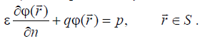 (6.41)
In the theory and practice of direct methods for solving such problems, a variational approach is often used, which allows the original problem of integrating a differential equation to be replaced by another, equivalent problem, consisting in finding the minimum of a certain functional. With this approach, the process of finding the solution can conditionally be divided into two stages, the first of which consists in constructing the functional equivalent to the original differential equation, and the second – in transforming this functional into a system of linear algebraic equations and solving it numerically.
Let us use this approach to solve the stated problem, and at its first stage we form a functional with respect to the unknown function (r) r ϕ, taking as a basis Poisson's equation (6.40) together with the boundary condition (6.41). To do this, we proceed as follows. Multiply the left and right
sides of equation (6.40) by some function v(r) r, which is continuous together with its two derivatives in V and satisfies the boundary conditions (6.41). Then integrate the left and right sides of the resulting equality over the volume V:
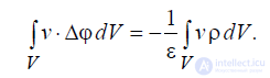
To further transform expression (6.42), let us use Green's first formula (B.27):

,
into which we make the following substitutions: v(r) r Ψ = and Φ = ϕ, which as a result gives:

and then, replacing the first term here using equality (6.42):
 . (6.43)
Now, using the boundary condition (6.41), let us find the normal derivative of the sought function:
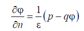
and substitute it into the last expression, which takes its final form:
 . (6.44)
The left side of the resulting equality represents a functional of
the unknown function (r) r ϕ, while its right side is expressed through known functions and quantities. Thus, we have constructed the functional we need through identical transformations of the original equation (6.40) and the given boundary conditions (6.41), which allows us to consider the first stage of solving the stated problem as completed.
Let us now proceed to the second stage of solving the problem, the goal of which is to transform expression (6.44) into a system of linear algebraic equations using the Bubnov-Galerkin method. To do this, we choose an infinite sequence of linearly independent basis functions n (r) r ψ, which are twice differentiable in the closed region V and satisfy the boundary conditions of our problem. If the sought function (r) r ϕ is represented as an expansion
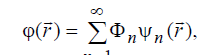 (6.45)
where Φn – are arbitrarily chosen constants, then it will also satisfy the boundary conditions of the problem, since equation (6.40) and boundary conditions (6.41) are linear.
In actual computations, expansion (6.45) must be finite, but then the new function
 (6.46)
will differ somewhat from (r) r ϕ. However, when the requirement
 (6.47)
is satisfied, one can always find such an N for which this difference does not exceed
the allowable value.
According to the Bubnov-Galerkin method, the coefficients Φn are determined from the requirement that equality (6.44) be satisfied when N (r)
r ϕ
is substituted instead of (r) r ϕ and n (r)
r ψ (n = 1,K,N) instead of v(r) r. Performing these operations, we arrive at the equality:

Now, interchanging the operations of integration and summation,
we obtain:
 (6.48)
The resulting expression represents a system of equations of order N with N unknowns Φn. This system of linear equations can
be written in matrix form:
 , (6.49)
where K and Q – are square matrices, Φ, F and P – are column matrices, the elements
of which are determined by the following relations:
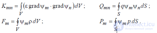 (6.50)
The solution of system (6.50) has the form:
 (6.51)
where −1 – is the matrix inversion operation.
Thus, we have found the coefficients of the expansion in series (6.46) of the unknown function N (r) r ϕ, which for sufficiently large N is close to the sought function (r) r ϕ, that is, we have found an approximate solution to the stated problem. At the same time, this solution has so far been obtained by us only formally, since the basis functions n (r)
r ψ have not been finally chosen, although we imposed fairly strict requirements on them. Now we proceed directly to the choice of these functions, which ultimately determines the name of the finite
element method.
To simplify the presentation, let us choose the basis functions using the example of a two-dimensional problem, i.e., when the sought electric field depends only on
two coordinates (for example, x and y), and equation (6.40), with ε = const, in a rectangular coordinate system takes the form:
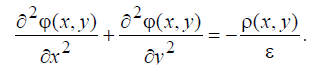 . (6.52)
The domain of definition of the function (r) r ϕ is now the area Ω on the plane xOy (rather than the volume V, as in the case of the three-dimensional problem), and its boundary – the contour ∂Ω (instead of the surface S). Therefore, boundary conditions (6.41) here
take the form:

Let us construct the system of basis functions ψN as follows. We divide
the region Ω into elements in the form of triangles, as a result of which it becomes covered by a grid with triangular cells (fig. 6.5,a). Let the total number of grid nodes be equal to M, of which N lie inside the region Ω, and the remaining L
are located on its boundary ∂Ω (M = N + L).
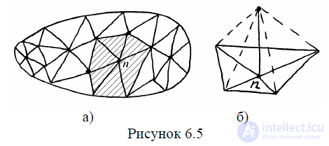
Now let us define the properties of the functions ψn (n = 1KM). Let each basis function ψn – be a piecewise-linear function, taking the value ψn =1 at the node numbered n and identically equal to zero throughout the entire region
Ω, except for several triangles having a common vertex at
the n-th node. Within the triangles adjoining the n-th node, the function varies linearly, decreasing from unity at their common vertex (the n-th node) to zero at the boundary of the polygon formed by them (shaded in fig. 6.5,a
). A graphical representation of the function ψn is a surface having the shape of a pyramid with apex at the n–th node (fig. 6.5,b) and base in the form of the aforementioned shaded polygon. Since
each triangle has three vertices, it will belong to three polygons, and consequently only three basis functions ψk, ψm and ψn can be nonzero inside it, whose indices k, m, n coincide with the numbers of the nodes that are the vertices of this triangle. Thus, the sought function can be written as the sum:
 . (6.53)
From the properties of the basis functions and equality (6.53), it follows that at the n–th node
the value of the sought function (rn) r ϕ is determined by the equality ϕ(rn) = Φn r. Consequently, the coefficients Φn (n = 1KM), determined from the solution of the system of linear equations (6.51), are the values of the sought function at the nodes
of the constructed grid. The function (r) r ϕ within each element is linear. For example, in a Cartesian coordinate system it can be described by
a function of the form:
ϕ(x, y) = ax + by + c,
where a, b and c – are coefficients uniquely determined by the coordinates of the nodes
and the coefficients Φn.
Thus, the solution of equation (6.24) has been found. The geometric interpretation of the solution is a surface composed of individual triangles. The only question that remains open is: into how many elements is it ne-
cessary to divide the region Ω for the solution to be acceptable to the user? An architect who needs to cover the spherical dome of a cathedral with triangular tiles solves an analogous problem. If a large tile size is chosen, the work can be done quickly and at low cost, but the dome will be faceted and will not resemble a sphere very much. If very small tiles are chosen, the dome will look smooth and beautiful, but the labor cost of making it will be high. Therefore, it is necessary to seek the optimal size of the flat surface element (tile), which, on the one hand, allows a spherical surface to be created with sufficient accuracy, and on the other hand, does not lead to excessive expenditure of time and resources. The same is true in the finite element method: to increase the accuracy of the solution, the area of the elementary cells must be reduced, which naturally increases the computational cost. And in this case, a compromise must be sought between acceptable solution accuracy and permissible computational resource costs. Therefore, within the framework of this method, a special strategy has been developed for choosing the optimal number of cells and their sizes. It involves a nonuniform partitioning of the entire region Ω under study, in which elements in different parts of the surface differ from one another in size. Where a sharp change in the sought function is expected, cells of smaller size are chosen than where the function changes fairly smoothly. This strategy makes it possible to achieve approximately uniform accuracy in reproducing the sought function throughout its entire domain of definition, while avoiding redundant computations.
The finite element method forms the basis of the electromagnetic field simulation program implemented in the PDE Toolbox application of the popular and powerful computer mathematics system MATLAB. It has proven to be very effective in solving many other applied problems as well, and not only in electrodynamics. The finite element method is currently developing intensively, and the range of its areas of application is continuously expanding.

Comments