
Lecture
Transformations in two-dimensional space are used in a variety of situations: so that individual parts of an object can be described in different coordinate systems; so that standard and repeating parts can be placed in arbitrary positions on a drawing or in space, including through the use of loops; so that symmetric parts of an object can be obtained without re-coding; for the directed deformation of shapes, bodies, and their parts; for changing the scale of a drawing, constructing projections of spatial images... From an analytical point of view, a transformation is a recalculation of coordinate values.
A point in the plane is represented by two coordinates: |x y|. The transformation matrix of a point looks like this:

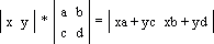
Below is the transformation of a point using a square matrix; here xn = xa + yc and yn = xb + yd are the new coordinates of the point after transformation:
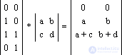
If a figure is represented as a set of points, its transformation can also be carried out. In the following example, four points are given: A(0, 0), B(1, 0), C(1, 1), D(0, 1), each of which, after transformation, maps respectively to A*(0, 0), B*(a, b), C*(a + c, b + d), D*(c, d):
Geometrically, this corresponds to a deformation of the figure:
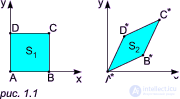
In this case, the area of the new figure equals the area of the old figure multiplied by the determinant of the transformation matrix: S2 = S1 * |ad - bc|.
Any coordinate system in which a point in two-dimensional (three-dimensional) space is represented using three (four) coordinates (P1, P2, P3(, P4)) is called a system of homogeneous coordinates. In general, for n-dimensional space, the number of homogeneous coordinates must be one greater: n + 1.
The use of homogeneous coordinates, in the general case, makes it possible to eliminate anomalies that arise when working in Cartesian coordinates, and to represent complex transformations as the product of several matrices.
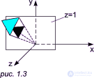
Geometric interpretation for the case of two-dimensional space: introducing a third coordinate equal to one can be interpreted as a transition into three-dimensional space, in which it is only allowed to work in the plane z = 1. One should imagine that the computer screen (the picture plane, the image plane) lies in the plane z = 1:
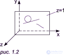
If the drawing goes beyond the section z = 1, the drawing is forcibly returned to this section — so that subsequent operations remain possible:
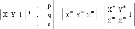
This operation is called normalization of homogeneous coordinates:

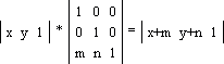
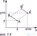
The transformation matrix contains the constants m and n, under whose action the point is shifted by m units along the x axis and by n units along the y axis:
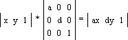
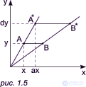
Due to the coefficients a and d of the transformation matrix, the coordinate values of the point (x, y) are increased (or decreased) by a factor of a and d along the x and y axes respectively:
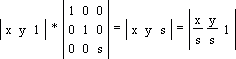
In this case, when s < 1, the coordinate values of the point (x, y) will increase by a factor of s; when s > 1, we get the opposite effect — a decrease in the coordinate values (x, y) by a factor of s.

Here q is the angle by which the point (x, y) is to be rotated. Note: the rotation occurs about the point (0, 0) of the Cartesian coordinate system, counterclockwise!
And now here is a small task for you. Try to rotate a triangle by an angle q = 90o, you can take any coordinates for the points. Our version is presented here.
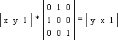
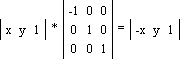
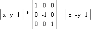
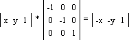
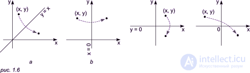
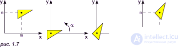
To carry out any complex transformation, it must be decomposed into basic operations. Rotation of a figure about an arbitrary point (m, n) by an arbitrary angle a consists of three basic operations: 1) translating the figure by the vector A(-m, -n) to align the point (m, n) with the origin of coordinates; 2) rotating the figure by the angle a; 3) translating the figure by the vector A'(m, n) to return it to its original position. Since a figure can be represented by a set of points, operations 1) - 3) can be performed sequentially for each point. Let us illustrate this with an example.
Suppose we want to rotate a triangle with coordinates A(x, y), B(x1, y1), C(x2, y2) about the point D(m, n) by the angle a. Let P-s be the matrix for translating a point by the vector A(-m, -n), Va be the matrix for rotation by the angle a, and Ps be the matrix for translating a point by the vector A'(m, n).
So, we have all the data necessary to carry out the complex transformation of the first point A(x, y):
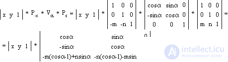
Exactly the same transformations must be carried out for the remaining two points of the triangle, substituting their corresponding coordinates in place of x and y (for the sequence of operations, see fig. 1.7). Thus, a complex operation is broken down into the simplest ones and is given by the product of the corresponding transformation matrices, and the order in which the matrices are multiplied significantly determines the result.

px + qy + 1 = H — the plane.
In the general case, the result changes if the matrices are swapped.
Matrices of consecutive operations can be multiplied separately, the main thing being not to change their order (see note 1).
Under the (affine) transformations described above, lines map to lines. Therefore, usually only the coordinates of the figure's vertices are recalculated, after which the corresponding vertices in the resulting figure are connected, just as in the original figure.
Suppose we have two lines: x + y = 1, 2x - 3y = 0, and we need to find their point of intersection. The solution can be found using matrices. Let us move all terms of the equations to the left-hand side: x + y - 1 = 0, 2x - 3y - 0 = 0; let us write the coefficients of the first equation into the first column of the matrix, and those of the second equation into the second column:

The condition under which two lines intersect looks as follows:
|x y 1| * M = |0 0 1|
To find the answer, both sides of the previous equation must be multiplied on the right by the inverse matrix M-1 (multiplying M and M-1 gives the identity matrix E):
|x y 1| * E = |0 0 1| * M-1
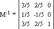
|x y 1| = |3/5 2/5 1|
Answer: the point of intersection of the lines is: x = 3/5, y = 2/5.
Everyone knows how a point is specified, but how are other figures specified? A circle is specified by three numbers: the x- and y-coordinates of the center and the radius; for an ellipse, in addition to the coordinates of the center, one must add the values of its two semi-axes and also the direction of one of the axes. The same figure can be specified in different ways, but usually those for which the number of parameters is minimal are singled out. This minimum number is called the "parametric number of the shape." When writing programs and algorithms for computer graphics, one needs to know the parametric numbers of the basic geometric shapes.
| Table of parametric numbers for some geometric shapes | ||
| Object | Dimensionality of space | Parametric number |
| Line segment in the plane | 2 | 4 |
| Line segment in space | 3 | 6 |
| Circle in space | 3 | 6 |
| Sphere | 3 | 4 |
| Arc of a circle in the plane | 2 | 5 |
| Rectangle in general position | 2 | 5 |
| Ellipse in general position | 2 | 5 |
| Ellipsoid | 3 | 9 |
| Second-order surface | 3 | 9 |
| Curve of a polynomial of degree n | 2 | n+1 |
"Logical parameters" may also be involved in specifying an object. In this case, one can limit oneself to the numbers 0 and 1, or set the parameter by the sign of a number. These parameters do not affect the parametric numbers of objects. For example, a point on a circle can be specified by the value of one of its coordinates (X or Y), but it will be necessary to indicate on which semicircle it may lie.
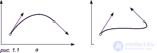
In computer graphics, it matters from which end a geometric component is traced, in which case the direction of tracing must be specified. This is needed to determine the visibility of sides. The direction of traversal of a body can be specified by the sign "+" or "-"; tangents can be used, but most often tangent vectors, or "direction vectors," are used. A vector in the plane can be specified by its two projections; tangent vectors have an arbitrary length — so one number would suffice, however for convenience projections are used. Fig. 1.1a shows an arc constructed from two endpoints and the tangent vectors drawn from them. This set (endpoints and tangent vectors) is one of the typical data configurations. If the direction of one of the vectors is reversed, we get the picture shown in fig. 1.1b.
Thus, two regions ("sides") can be distinguished for a line: a "positive" one, on which the normal vectors will lie, and a "negative" one. Lines drawn on a surface divide the surface, and surfaces divide space. This technique is used to solve problems of applying hatching to various elements of a drawing, determining whether a point belongs to a body of complex shape, and identifying visible or bounded parts and surfaces.
Let us touch on two different methods of representing geometric objects in a computer.
The first method is analytical models. An analytical model is a set of numbers and, if necessary, logical parameters that act as coefficients and other quantities in the equations and analytical relations defining an object of a given type. For example, for a circle the basic form of the analytical model is the coordinates of the center and the radius, related by the well-known relation: (x - xc)2 + (y - yc)2 - R2 = 0.
A circle, like many other objects, can be specified in parametric form, where, besides the coordinates, there is one more variable quantity — the parameter. The parametric specification of shapes is widely used in computer graphics.
The second method of numerical modeling of geometric objects in a computer is coordinate models. In simple cases, these are sets of points that belong to the objects and are specified by coordinates. For curves and polylines, the points are arranged in the same order as on the line. Ordering the points of a surface is a more complex task: in most cases the points are sequentially arranged along lines drawn on the surface.
Coordinate models have several varieties:
Many graphics devices have linear interpolators. That is, if these are devices of the trajectory type, the elements of the image are represented as coordinate models supplemented with control commands. The points specified in them in sequence are connected by straight-line segments, so that all curves are represented as polylines with small links. This principle makes it possible to replace objects that are diverse and analytically complex with sets of simple objects. After this, the same algorithms can be used to perform operations on them. For some algorithms, successive points can be connected by arcs of various curves, which makes it possible to reduce the number of reference points in the model without reducing the accuracy of the representation.

Comments