
Lecture
The main goal is to describe a curve using a sequence of curve segments. As a rule, all vector editors have a similar interface for editing curves. To change the shape of a curve, the user can use a special tool to change the position of a node and the ends of the vectors adjoining it. In order for the curve to have no kinks at the points where curve segments join, their adjoining vectors must be collinear. (fig. 2.1).
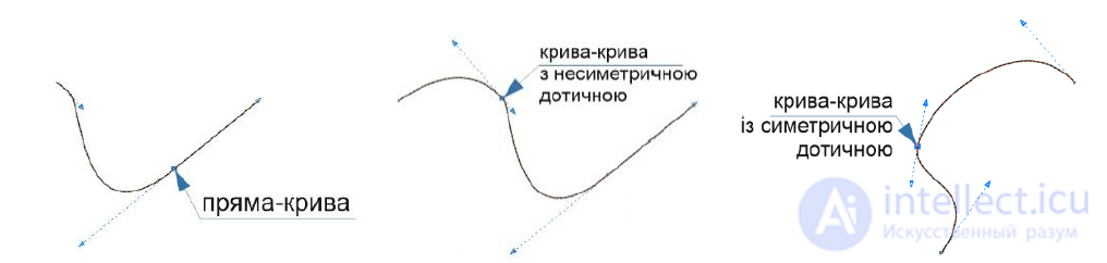
Fig. 2.1 – editing curves in CorelDraw
Below, for the description we will use the general notation 𝐶(𝑖) -continuity. Curves are said to be 𝐶(0)-continuous if they have no breaks, and curves are said to be 𝐶(1) -continuous if, in addition, their adjoining (derivatives) are continuous.
There are two main ways of representing curves: by means of functions of the variables 𝑥, 𝑦, 𝑧, and by means of functions of some parameter 𝑡.
In the first case, in order to determine points (𝑥,𝑦,𝑧) on the curve, one has to deal with functions of the form
𝑥=𝑥, 𝑦=𝑓(𝑥), 𝑧=𝑔(𝑥). (1)
This representation entails many complications: at some point on the curve, the tangent of the slope angle may turn out to be infinite. It is also not simple to check whether a point belongs to a given segment of the curve defined by its start and end points.
With a parametric representation of three-dimensional curves, these problems are substantially simplified, since with such a representation it is easy to describe closed,
multivalued functions, and, moreover, instead of tangents of slope angles, adjoining vectors are used, which are never infinite.
A parametric cubic curve is a curve in which 𝑥, 𝑦, 𝑧 are third-order (cubic) polynomials with respect to some parameter 𝑡. Since we are considering finite segments of the curve, without loss of generality we can restrict the range of the parameter and take it that 0 ≤ 1.
So

The derivatives of the functions 𝑥(𝑡), 𝑦(𝑡), 𝑧(𝑡) with respect to the parameter 𝑡 have the same form:

The three derivatives define a tangent vector. The tangents of the curve's slope angles are given as the ratio of the components of this vector:

The slope angles do not depend on the length of the adjoining vector. If we multiply the derivatives by k, we obtain
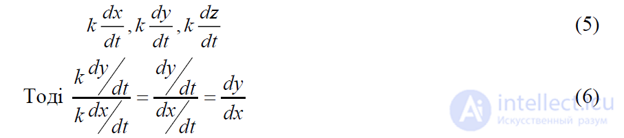
In searching for ways to determine 𝑎𝑥, 𝑏𝑥, 𝑐𝑥, 𝑑𝑥, below we will deal
only with the derivatives of 𝑥(𝑡). For 𝑦(𝑡) and 𝑧(𝑡) the derivatives and final formulas are analogous
to the formulas for 𝑥(𝑡), and we will not present them.
Why do we consider cubic curves in particular? Because for curve segments there
exists no lower-order representation that would ensure, at the point where
curves join one another, continuity of the segments' position and slope, while at the same time
guaranteeing that the endpoints of the curve segment pass through the given points.
A parametric cubic polynomial with four coefficients is the lowest-degree parametric curve that, given an appropriate
choice of coefficients, can satisfy four conditions (the position of each of the segment's ends and
the tangent vectors at them).
We will consider only three ways of describing parametric bicubic curves:
the Hermite method, in which the positions of the curve's endpoints and the tangent
vectors at them are specified; the Bezier method, in which the position of the curve's endpoints is specified,
and for the implicit task of the adjoining vectors at these points, two other points are used, generally not lying on the curve; the B-spline method, in which the endpoints
do not lie on the curve, as a result of which both the first and second derivatives turn out to be continuous at the ends of the segment. (fig. 4)
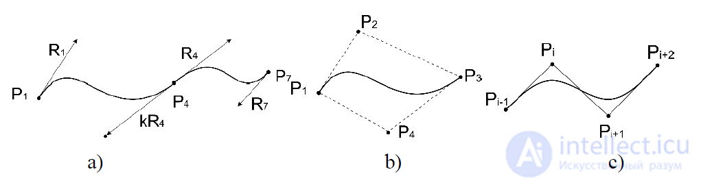
Fig. 2.2 – forms of specifying bicubic curves: a – Hermite; b – Bezier, c – B-spline.
In the Hermite form, the endpoints and the adjoining vectors to the curve at these
points are specified (fig. 2.2-a). Let us specify points 𝑃1 and 𝑃4 and adjoining vectors 𝑅1 and 𝑅4 (the points are given the indices 1 and 4, rather than 1 and 2, for compatibility with the expressions used
in constructing curves by the Bezier and B-spline methods). It is required to find the coefficients 𝑎𝑥, 𝑏𝑥, 𝑐𝑥, 𝑑𝑥 from expression (2) that satisfy the conditions

We use the index x to refer to the x-components of the points and adjoining vectors. Rewriting the expression for x(t), we obtain.
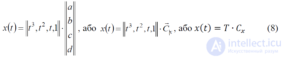
where T is the row vector of powers of 𝑡, and 𝐶𝑥 is the column vector of coefficients of 𝑥(𝑡).
Let us write conditions (7) using equation (8).

To write the expression for the constraints on the adjoining vectors, let us differentiate
expression (9) with respect to 𝑡 and obtain:

Expressions (9) and (10) can be combined into a single matrix equation
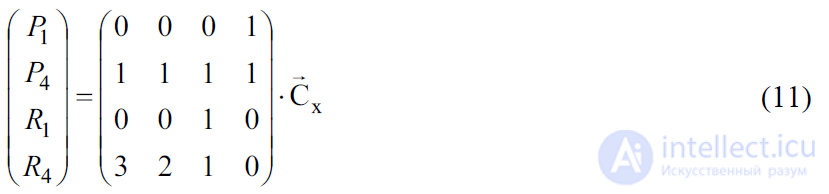
Having found the inverse matrix, we obtain the expression for 𝐶𝑥, if we set:
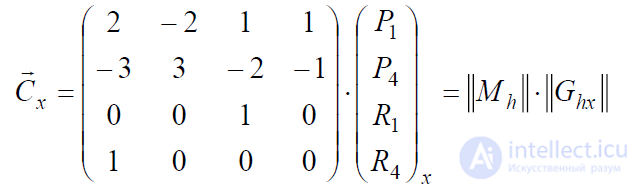
Here ‖𝑀ℎ‖ (𝑀ℎ) denotes the Hermite matrix, and ‖𝐺ℎ‖ (𝐺ℎ) denotes the Hermite geometric vector.
Substituting this result into (8), we obtain:

If 𝑃1, 𝑃4, 𝑅1, 𝑅4 are given, one can determine 𝑥(𝑡), 𝑦(𝑡), 𝑧(𝑡) for 0 ≤ 𝑡 ≤ 1 and
find all the points on the segment of the cubic curve from 𝑃1 to 𝑃4, whose adjoining vector at the starting point equals 𝑅1, and at the endpoint – 𝑅4.

Multiplying (14) by 𝐺ℎ𝑥, we obtain:

The four functions of the variable 𝑡 in form (15) are called blending functions,
since the first two are used to join points 𝑃1 and 𝑃4, while
the other two are used to join the vectors 𝑅1 and 𝑅4, whereby a "smoothed" merging of
𝑥(𝑡) is achieved.
The Bezier form of description is very close to the Hermite form, but differs in how the adjoining vectors are specified at the endpoints.
The adjoining vectors at the endpoints are specified by the segments [𝑃1𝑃2] and [𝑃3𝑃4].
In particular, the tangent vectors of the Hermite form 𝑅1 and 𝑅4 were defined in such a way as to correspond to the four Bezier points 𝑃1, 𝑃2, 𝑃3, 𝑃4:

Therefore, the relationship between the Hermite matrix and the Bezier matrix Gb is written, in the general case, as follows:
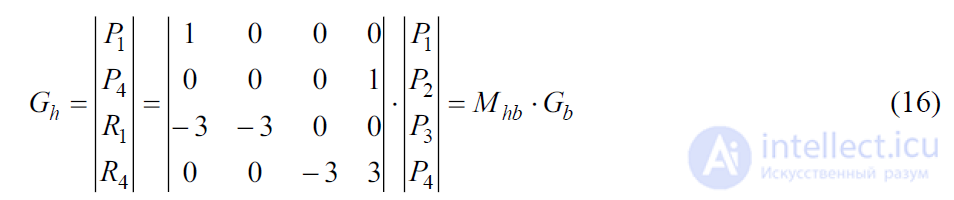
Substituting (16) into (13), we find: x(t)=T·Mh·Ghx = T·Mh·Mhb·Gbx
Denoting by Mb the product Mh·Mhb, we obtain the expression
x(t)=T·Mb·Gbx, which now has the Bezier form. x(t)=T·Mb·Gbx

Continuity at the junction of two Bezier curves is ensured by satisfying the equality of the vectors P3P4 = k P4P5.
The Bezier form, owing to its two properties, is used in computer
graphics more often than the Hermite form. First, specifying (and changing) the tangent
vectors in the form of two points interactively is more convenient than doing so explicitly. Second, the four control points define a convex polygon
(convex hull), inside which the Bezier curve lies. The convex hull turns out to be useful when clipping a curve against a window or a viewing volume.
A spline was the name given to a flexible metal ruler — a universal curve template,
which was used to smoothly connect individual points on a drawing,
that is, for graphical interpolation. Moreover, the curve describing the deformation
of a flexible ruler fixed at individual points is a spline. Thus, the flexible
ruler is a physical model of a spline function (or, conversely, a spline function is a mathematical model of a flexible ruler).
A B-spline (basis spline) is a spline function having minimal support for
a given degree, order of smoothness, and domain of definition.
The fundamental theorem states that an arbitrary spline function of a given
degree, smoothness, and domain of definition can be represented as a linear combination of B-splines of the same degree and smoothness on the same domain of definition.
A curve represented as a cubic B-spline, in the general case,
need not pass through any of the control points; however, it is continuous and, moreover,
its adjoining vector and curvature are continuous (i.e., the first and second derivatives of the curve are continuous at the endpoints), unlike the Hermite and Bezier forms, for which at the
endpoints only the first derivatives are continuous, and which pass through the control points. Thus, it can be said that the B-spline form is "smoother" than the other forms. The term spline comes from the name of the long flexible metal rulers used to lay out the surfaces of aircraft and ships on drafting plans.
A metal spline, if not heavily stressed, also has second-order continuity. A B-spline is described by the following formula:
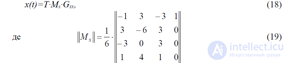
When approximating control points P1, P2, ... Pn with a sequence of B-splines,
we will apply geometric matrices between each pair of neighboring points. For approximation in the interval close to points Pi and Pi+1, (fig. 2.2-c) the following is used
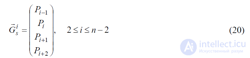
The convex hull property of the Bezier curve also holds for curves in the B-spline form: the convex hull of the curve in the approximated interval Pi - Pi+1
is the same as for the four control points used to generate the curve: Pi - 1, Pi, Pi+1, Pi+2
The Hermite form is suitable for approximating already existing surfaces, when it is necessary to achieve both correspondence of points and correspondence of vectors, whereas representation in the form of B-splines is convenient for approximating points and achieving
C(2)-continuity. The Bezier and B-spline forms are suitable for interactive work.
Both of these forms possess the convex hull property. Note
that a curve originally specified in one form can be converted into another form by writing the geometric vector of the first form in terms of the second.

Comments