
Lecture
2.1 The coordinate method
The coordinate method was introduced in the seventeenth century by the French mathematicians R. Descartes and P. Fermat. Analytic geometry, which can be regarded as the foundation of computer graphics (CG), is based on this method. In modern CG the coordinate method is widely used.
2.1.1. Coordinate transformation First let us consider general questions of coordinate transformation. Suppose an n-dimensional coordinate system is given in the basis (k1, k2,.... kn), which describes the position of a point in space by means of the numerical values ki. In CG the two-dimensional (n = 2) and three-dimensional (n = 3) coordinate systems are used most often. If we define another, N-dimensional, coordinate system in the basis (m1, m2,..., m) and pose the problem of determining the coordinates in the new system given the coordinates in the old one, the solution (if it exists) can be written as follows:
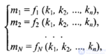
where fi is the recalculation function for the i-th coordinate, whose arguments are the coordinates in the system ki. One can also pose the inverse problem: given the known coordinates (m1, m2,.... m), determine the coordinates (k1, k2,..., kn). We write the solution of the inverse problem as follows:
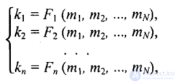
where Fi are the functions of the inverse transformation. If the dimensions of the coordinate systems do not coincide (n ≠ N), it is most often impossible to carry out an unambiguous coordinate transformation. For example, from two-dimensional screen coordinates it is impossible, without additional conditions, to unambiguously determine the three-dimensional coordinates of the displayed objects. Linear transformations are conveniently written in matrix form:
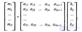
Here the coefficient matrix (aij) is multiplied by the column matrix (ki), and as a result we obtain the column matrix (mi)
We will continue to make frequent use of matrix multiplication further on, so let us make a brief excursion into matrix algebra. For two matrices —
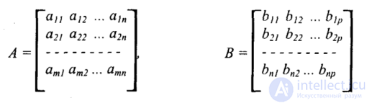
matrix A of size (m x n) and B — (n x p): the matrix product is the matrix C = AB of size (m x p):
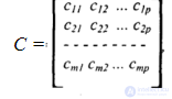
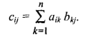
C = , for which the elements cij are calculated by the formula
The simplest two-dimensional transformations
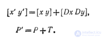
Points on the xy-plane can be moved to new positions by adding translation constants to the coordinates of those points. For each point P(x, y), which is moved to a new point P'(x, y) by shifting Dx units parallel to the x axis and Dy units parallel to the y axis, we can write the equations:

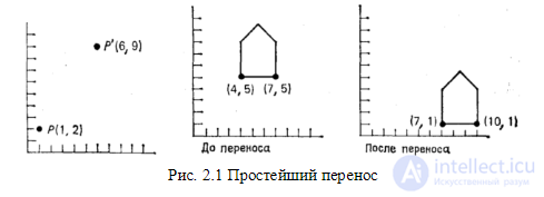
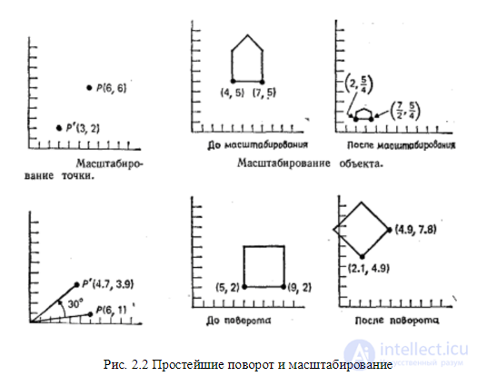
Figure 2.1 shows a point with coordinates (1, 2) that is displaced by the distance (5, 7), turning into the point (6, 9). Defining the row vectors

we can rewrite this equation in vector form, or more briefly
An object can be translated by applying the equation derived above to each of its points. However, since every segment describing the object consists of an infinite number of points, this process would take an infinitely long time. Fortunately, all points belonging to a segment can be translated by moving only the segment's endpoints and then drawing a new segment between the resulting points. This also holds for scaling (stretching) and rotation. Figure 2.1 shows the result of applying a translation by the distance (3, -4) to the outline of a house
Points can be scaled (stretched) by a factor of Sx along the x axis and by a factor of Sy along the y axis, obtaining new points as a result by means of multiplication. Defining S as , we can write it in matrix form, or . In Figure 2.2 a single point (6, 6) is scaled with coefficients 1/2 along the X axis and 1/3 along the Y axis. The same figure shows the outline of a house scaled with coefficients 1/2 along the x axis and 1/4 along the y axis. Note that scaling is performed relative to the origin of coordinates; as a result of the transformation the house has become smaller and closer to the origin. If the scale factors had been greater than 1, the house would have grown larger and moved farther from the origin. Methods for performing scaling relative to points other than the origin are considered in one of the subsequent sections of the chapter. The proportions of the house have also changed · non-uniform scaling was applied, in which Sx ≠ Sy. Uniform scaling, for which Sx = Sy, does not affect the proportions. Points can be rotated by an angle θ relative to the origin of coordinates, as shown in Figure 2.2 for the point P (6, 1) and an angle θ = 30°. Mathematically, rotation is defined as follows: In matrix form we have , or , where R denotes the rotation matrix. Figure 2.2 shows a square rotated by 45°. As in the case of scaling, rotation is performed relative to the origin of coordinates.
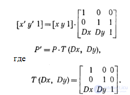
Homogeneous coordinates and the matrix representation of two-dimensional transformations The transformations of translation, scaling, and rotation are written in matrix form as . Unfortunately, translation is implemented separately (by addition) from scaling and rotation (by multiplication). It would be desirable to represent them in such a way that all three of these elementary transformations could easily be combined together. This section shows below how this can be done. If we express points in homogeneous coordinates, then all three transformations can be implemented by means of multiplication. Homogeneous coordinates were introduced in geometry and were subsequently used in graphics. Many graphics subroutine packages and some display processors work with homogeneous coordinates and transformations on them. In some cases these coordinates are used directly by the application program when specifying parameters for the graphics package; in others they are used only inside the package itself and are not accessible to the programmer. In homogeneous coordinates a point P(x, y) is written as P(W·x, W·y, W) for any scale factor W≠0. Here, if the representation of a point in homogeneous coordinates P(X, Y, W) is given, its two-dimensional Cartesian coordinates can be found as x = X/W and y = Y/W. In this chapter W will always equal 1, so the division operation is not required. Homogeneous coordinates can be represented as the embedding of a two-dimensional plane, scaled by a factor W, into the plane z = W (here z = 1) in three-dimensional space. Points are now described by three-element row vectors, so the transformation matrices by which a point vector is multiplied to obtain another point vector must have size 3x3. The translation equations are written as a homogeneous-coordinate transformation matrix as follows:
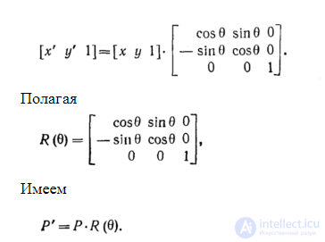
What happens if a point P is translated to a point P' by a distance (Dx1, Dy1), and then to P" by a distance (Dx2, Dy2)? Intuitively, the expected result in this case is a total translation by the distance (Dx1+Dx2, Dy1+Dy2). To prove this, let us write the data as . We now obtain: The matrix product T(Dx1, Dy1)·T(Dx2, Dy2) is . Indeed, the resulting translation is (Dx1+Dx2, Dy1+Dy2). The matrix product is in various cases called the union, join, concatenation, and composition of the matrices T(Dx1, Dy2) and T(Dx2, Dy2). In this chapter we will use the term composition. The scaling equations are written in matrix form as . Defining , we have . Just as successive translations are additive, we can expect that successive scalings will be multiplicative. If we are given , then we obtain: The matrix product S(Sx1, Sy1)·S(Sx2, Sy2) is . Thus, scalings are indeed multiplicative. And finally, the rotation equations can be represented as follows:
Composition of two-dimensional transformations
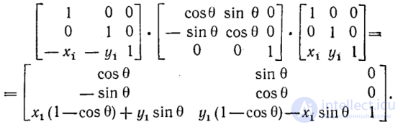
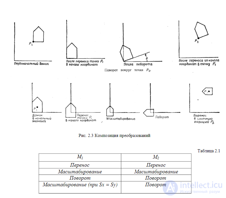
The concept of composition was introduced in the previous section. In this section we show how composition of transformations can be used to combine the fundamental matrices R, S, and T in order to obtain the desired overall results. The main advantage of combined transformations is that it is more efficient to apply a single resulting transformation to a point than a series of transformations one after another. Consider, for example, the rotation of an object relative to some arbitrary point Pi. Since we know only how to rotate about the origin, let us break the original (difficult) problem down into three easier tasks. Thus, in order to perform a rotation relative to the point Pi, it is necessary to carry out three elementary transformations in sequence: 1. Translation, by which the point Pi is moved to the origin. 2. Rotation. 3. Translation, by which the point is moved back from the origin to its original position Pi. This sequence is shown in Figure 2.3, in which the outline of a house is rotated about the point Pi(x, y). The first translation is performed by (-x1, -y1), while the subsequent one — by (x1, y1) — is its inverse.
The result differs substantially from what would be obtained if rotation alone were applied. The resulting transformation has the form
This composition of transformations by matrix multiplication serves as an example of how the use of homogeneous coordinates simplifies the task. Using a similar approach, an object can be scaled relative to an arbitrary point Pi: translate Pi to the origin, scale, then translate back to the point Pi. The resulting transformation in this case will have the form
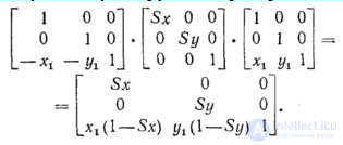
Suppose we need to scale, rotate, and position at the desired location the house shown in Figure 2.3, where the point P1 is the center of rotation and scaling. The sequence of transformations consists of translating the point P1 to the origin, performing the scaling and rotation, and then translating from the origin to the new position P2 at which the house should end up (this sequence is shown in Figure 2.3). The data structure containing this transformation may store the scale factor(s), the rotation angle, and the translation amounts, or the matrix of the resulting transformation may be recorded directly:

If it is known that M1 and M2 represent elementary translation, scaling, or rotation, under what conditions are M1 and M2 commutative? In general, matrix multiplication is non-commutative. However, it is easy to show that in the following particular cases commutativity does hold (in these cases one need not worry about the order of matrix multiplication – see Table 2.1).
Matrix representation of three-dimensional transformations
Just as two-dimensional transformations are described by 3x3 matrices, three-dimensional transformations can be represented by 4x4 matrices. A three-dimensional point (x, y, z) is then written in homogeneous coordinates as (W·x, W·y, W·z, W), where W≠0. If W≠1, to obtain the three-dimensional Cartesian coordinates of the point (x, y, z) the first three homogeneous coordinates are divided by W. In particular, it follows from this that two points H1 and H2 in homogeneous-coordinate space describe the same point of three-dimensional space if and only if H1=cH2 for some nonzero constant c. The three-dimensional coordinate system used in this book is right-handed (Fig. 2.4). Let us adopt the convention according to which we consider as positive those rotations for which (when viewed from the end of the positive half-axis toward the origin) a 90° counterclockwise rotation carries one positive half-axis into another. Based on this convention we construct the following table, which can be used for both right-handed and left-handed coordinate systems
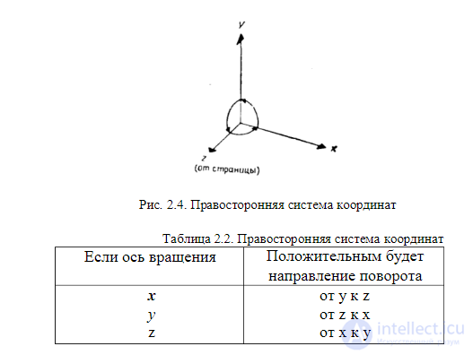
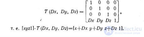
We use a right-handed coordinate system here because it is well known to most people, although in three-dimensional graphics a left-handed system is often more convenient, since it is easier to imagine as being overlaid on the surface of a display screen. This allows a natural interpretation of the fact that points with larger z values are farther from the observer. Note that in a left-handed system, positive rotations are those performed clockwise when viewed from the end of the positive half-axis toward the origin. Three-dimensional translation is a simple extension of the two-dimensional case:
Scaling is extended in an analogous way:
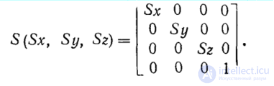
Indeed, . Two-dimensional rotation is at the same time a three-dimensional rotation about the z axis. In three-dimensional space, rotation about the z axis is described by the expression . This is easy to check: as a result of a 90° rotation of the vector [1 0 0 1], which is the unit vector of the x axis, the result should be the unit vector [0 1 0 1] of the y axis. Computing the product we obtain the predicted result [0 1 0 1]. The rotation matrix about the x axis has the form . The rotation matrix about the y axis is written as . The columns (and rows) of the upper-left 3x3 submatrix of the matrices Rz, Rx, and Ry are mutually orthogonal unit vectors, whose interpretation is the same as in the two-dimensional case. All these transformation matrices have inverse matrices. The inverse of matrix T is obtained by substituting a minus sign before Dx, Dy, and Dz; the inverse of S is obtained by replacing Sx, Sy, and Sz with their reciprocal values, and for each of the three rotation matrices — by choosing a negative rotation angle.
Composition of three-dimensional transformations
By combining elementary three-dimensional transformations, other transformations can be obtained. This section shows how to do this. The task consists of transforming the segments P1P2 and P1P3 (Fig. 2.5) from an initial position to a final one. The point P1 is translated to the origin, P1P2 is placed along the negative x half-axis, and P1P3 is placed in the yz plane, in the half where the y axis is positive. The transformation does not affect the lengths of the segments. As before, let us break the complex task down into simpler ones. In this case the transformation can be performed in four steps: 1. Translate the point P1 to the origin. 2. Rotate about the y axis until P1P2 coincides with the yz plane. 3. Rotate about the x axis until P1P2 coincides with the negative z half-axis. 4. Rotate about the z axis until P1P3 coincides with the yz plane. Step 1. Translate P1 to the origin:
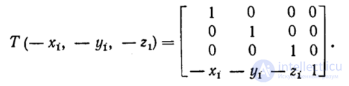
Applying T to P1, P2, and P3 gives . Step 2. Rotation about the y axis. Figure 2.5 shows the segment P1P2 after step 1 and the projection of P1P2 onto the xz plane. The rotation is performed by a positive angle θ, for which , where . Then . As expected, the x-component of P2 equals zero. Step 3. Rotation about the x axis. Figure 2.6 shows the segment P1P2 (Fig. 2.5. Composition of transformations) after step 2. The rotation is performed by a negative angle φ, for which , where . The notation denotes the length . The result of the rotation at step 3 is , i.e., now coincides with the negative z half-axis. Step 4. Rotation about the z axis. Figure 2.6 shows and after step 3, when P2''' lies on the negative z half-axis and P3''' is at the point . The rotation is performed by a positive angle , for which . Step 4 is the last step, after which the final result shown in Figure 2.6 is obtained. The resulting matrix
describes the sought transformation, where . (Fig. 2.6. Completion of the composition of transformations) Transformation of objects The transformation of objects can be described as follows. Let any point belonging to a given object have coordinates (k1, k2,..., kn) in an n-dimensional coordinate system. Then the transformation of an object can be defined as a change in the positions of the object's points. The new position of a point in space corresponds to new coordinate values (m1, m2,..., mn). The relationship between the old and new coordinates for all points of the object (m1, m2,..., mn) = F(k1, k2,..., kn) is what defines the transformation of the object, where F is the transformation function. Transformations of objects can be classified according to the type of transformation function and the type of coordinate system. For example, the transformation of objects in the plane can be defined as follows: . In three-dimensional space: . Transformation as a change of coordinate systems We consider the transformation of a set of points belonging to an object into some other set of points, where both of these sets are described in one and the same coordinate system. Thus the coordinate system remains unchanged, while the object itself is transformed relative to the origin until the desired size is obtained. Another equivalent way of describing a transformation is a change of coordinate systems. This approach turns out to be useful when it is desirable to gather together many objects, each of which is described in its own local coordinate system, and express their coordinates in a single global coordinate system. There is also a third approach, in which the global coordinate system is changed relative to the local coordinate system of the object (see Fig. 2.7)
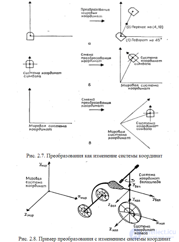
Describing all objects (symbols) in the world coordinate system and then placing them at the desired location leads, to some extent, to an unrealistic image, since all the symbols were initially defined one on top of another in the same world coordinate system. It is more natural to assume that each symbol is defined in its own coordinate system and is then scaled, rotated, and translated by a coordinate transformation into a new world coordinate system. The second approach is easy to imagine as compressing or stretching, rotating, and positioning, on the world coordinate plane, individual sheets of paper, each of which has a symbol drawn on it (or, conversely, compressing or stretching, rotating, and moving the plane relative to each of the sheets of paper). Mathematically, both approaches are identical. The approach based on changing coordinate systems is convenient in cases where additional information is given for sub-objects in their local coordinate systems. For example, if torque is applied to the front wheel of a tricycle (Fig. 2.8), all of its wheels will rotate. We need to determine how far the bicycle will move in space as a whole. This task is more complex than the one associated with placing symbols, since it requires several successive changes of coordinate systems. At the initial moment, the coordinate systems of the bicycle and of its front wheel are given relative to the world
coordinate system. As the bicycle moves forward, the front wheel rotates about the z axis of the wheel's coordinate system, and at the same time the coordinate systems of the wheel and of the bicycle are translated relative to the world coordinate system. The coordinate systems of the wheel and of the bicycle are linked to the world coordinate system by means of time-dependent translations along the x and y axes and a rotation about the y axis. The coordinate systems of the bicycle and of the wheel are linked to each other by means of a time-dependent rotation about the y axis, caused by the turning of the handlebars. (The coordinate system of the bicycle is attached to the frame of the bicycle, not to the handlebars). 2.1.2 Affine transformations in the plane This is a particular case of transformations that is quite often used in the creation of graphics packages. Let us define some two-dimensional coordinate system (x, y). An affine transformation in the plane is described by the formulas , where A, B, ..., F are constants. The value (X, Y) can be regarded as coordinates in the new coordinate system. The inverse transformation of (X, Y) into (x, y) is also affine: . An affine transformation is conveniently written in matrix form. The constants A, B, ..., F form a transformation matrix which, when multiplied by the column matrix of coordinates (x, y), gives the column matrix (X, Y). However, in order to take into account the constants C and F, it is necessary to move to so-called homogeneous coordinates — we add one more row to the coordinate matrices: . Now let us consider particular cases of the affine transformation. 1. Parallel shift of coordinates (Fig. 2.9). Fig. 2.9. Parallel shift of coordinates In matrix form . Inverse transformation: 2. Stretching-compression of the coordinate axes (Fig. 2.10)
Inverse transformation: . The coefficients kx and ky can be negative. For example, kx = -1 corresponds to a mirror reflection relative to the y axis. 3. Rotation (Fig. 2.11). Fig. 2.11. Rotation The inverse transformation corresponds to a rotation of the system (X, Y) by the angle (-α). Properties of the affine transformation. • Any affine transformation can be represented as a sequence of operations from among the simplest ones listed: shift, stretching/compression, and rotation. • The straightness of lines, the parallelism of lines, the ratio of the lengths of segments lying on the same line, and the ratio of the areas of figures are preserved. Three-dimensional affine transformation Let us write it as a formula: , where A, B, ..., N are constants. Let us also give it in matrix form:
For three-dimensional space, any affine transformation can likewise be represented by a sequence of the simplest operations. Let us consider them. 1. Shift of the coordinate axes by dx, dy, dz respectively: 2. Stretching/compression by kx, ky, kz. 3. Rotations. It can be said that in three-dimensional space there are more varieties of rotation compared with two-dimensional space. Let us consider several particular cases of rotation. Rotation about the x axis by the angle φ (Fig. 2.12). Fig. 2.12. Rotation about the X axis Rotation about the y axis by the angle ψ (Fig. 2.13, top). Rotation about the z axis by the angle γ (Fig. 2.13, bottom).
2.2 Projections When using any graphics devices, projections are normally used. A projection specifies a way of mapping objects onto a graphics device. We will consider only projections onto a plane. Projection is the mapping of points given in a coordinate system of dimension N onto points in a system of lower dimension. Projectors (projecting rays) are line segments running from the center of projection through each point of the object to their intersection with the projection plane (the picture plane). 2.2.1 World and screen coordinates When displaying spatial objects on a screen or on a sheet of paper by means of a printer, it is necessary to know the coordinates of the objects. We will consider two coordinate systems. The first is world coordinates, which describe the true position of objects in space with a given accuracy. The second is the coordinate system of the display device, in which the image of the objects is output in a given projection. Let us call the coordinate system of the graphics device screen coordinates (although this device need not necessarily resemble a computer monitor). Let the world coordinates be three-dimensional rectangular coordinates. Where the origin of coordinates should be placed, and what the units of measurement along each axis will be, is not very important to us right now. What matters is that for display purposes we will know some numerical values of the coordinates of the objects being displayed. To obtain an image in a given projection it is necessary to compute the coordinates of the projection. To synthesize an image on the plane of the screen or paper, we use a two-dimensional coordinate system. The main task is to specify the coordinate transformation from world to screen coordinates. 2.2.2 Basic types of projections The display of objects on a plane (the display screen) is associated with the geometric operation of projection. In computer graphics several types of projection are used, but there are two main types: parallel and central. A bundle of projecting rays is directed through the object onto the picture plane, on which the coordinates of the intersections of the rays (or lines) with this plane are subsequently found. Fig. 2.14. Basic types of projections In central projection, all lines originate from a single point.
In parallel projection, it is assumed that the center of the rays (lines) is infinitely distant, and the lines are parallel. Each of these two main classes is further divided into several subclasses depending on the relative position of the picture plane and the coordinate axes.
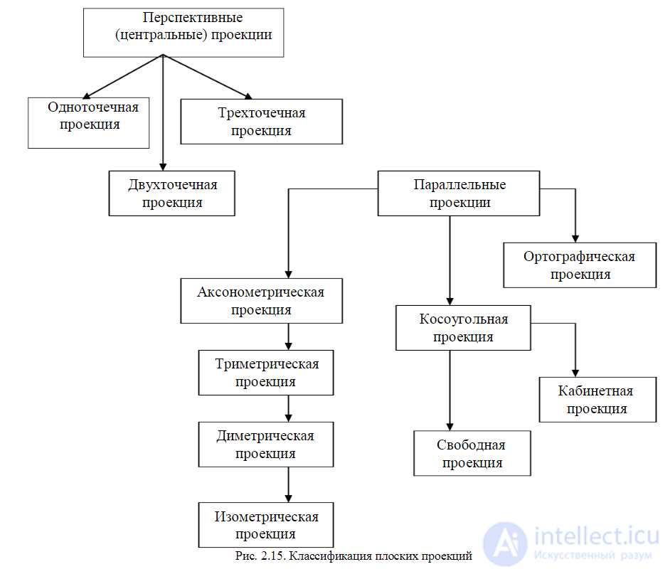
For parallel projections the center of projection is located at infinity from the projection plane: orthographic (orthogonal), axonometric (rectangular axonometric) — the projectors are perpendicular to the projection plane, which is positioned at an angle to the principal axis, oblique (oblique axonometric) — the projection plane is perpendicular to the principal axis, and the projectors are positioned at an angle to the projection plane. For central projections the center of projection is at a finite distance from the projection plane. So-called perspective distortions occur.
Orthogonal projections (main types) Fig. 2.16. Orthogonal projections 1. Front view, main view, frontal projection (onto the back face V), 2. Top view, plan, horizontal projection (onto the bottom face H), 3. Left view, profile projection (onto the right face W), 4. Right view (onto the left face), 5. Bottom view (onto the top face), 6. Rear view (onto the front face). The matrix of the orthogonal projection onto the YZ plane along the X axis has the form: 1 0 0 0 0 1 0 0 0 0 1 0 0 0 0 XP. If the plane is parallel, this matrix must be multiplied by the shift matrix, giving: 1 0 0 p 0 1 0 0 0 0 1 0 0 0 0 XP, where p is the shift along the X axis; For the ZX plane along the Y axis: 1 0 q 0 0 1 0 0 0 0 0 0 0 0 0 XP, where q is the shift along the Y axis; For the XY plane along the Z axis:
In axonometric projection, the projecting lines are perpendicular to the plane of the picture. Isometry — all three angles between the normal of the picture and the coordinate axes are equal. Dimetry — two of the angles between the normal of the picture and the coordinate axes are equal. Trimetry — the normal vector of the picture plane forms different angles with the coordinate axes. Each of these three types of projection is obtained by a combination of rotations followed by parallel projection. When rotating by the angle β about the Y axis (ordinate), by the angle α about the X axis (abscissa), and subsequently projecting along the Z axis (applicate), the matrix arises. Isometric projection Fig. 2.17. Isometric projections Dimetric projection Fig. 2.18. Dimetric projections
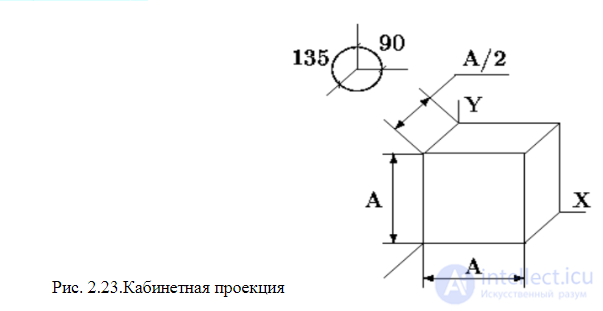
Oblique projections A classic example of a parallel oblique projection is the cabinet projection (Fig. 2.26). This projection is often used in mathematical literature for drawing three-dimensional shapes. The y axis is depicted tilted at an angle of 45 degrees. Along the y axis the scale is 0.5, and along the other axes the scale is 1. Let us write the formulas for computing the coordinates of the projection plane. Here, as before, the Ypr axis points downward. For oblique parallel projections, the projecting rays are not perpendicular to the projection plane. Fig. 2.19. Oblique projections Now let us turn to central projection. Since for it the projecting rays are not parallel, we will consider a central projection normal if its principal axis is perpendicular to the projection plane. For a central oblique projection, the principal axis is not perpendicular to the projection plane. Let us consider an example of a central oblique projection that shows all vertical lines of the displayed objects as parallel lines. Let us position the projection plane vertically, and specify the viewing angle by the angles α, β, and the position of the vanishing point (Fig. 2.21). Fig. 2.21. Vertical central oblique projection: a – position of the projection plane, b – view from the left end of the projection plane Let us assume that the Z axis of the view coordinates is perpendicular to the projection plane. The center of the view coordinates is at the point (xc, yc, zc). Let us write the corresponding view transformation:
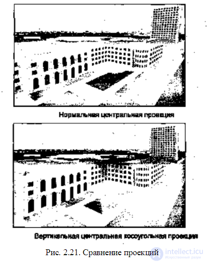
As with the normal central projection, the vanishing point of the projecting rays is located on the Z axis at a distance Zk from the center of the view coordinates. It is necessary to take into account the tilt of the principal axis of the oblique projection. To do this it is enough to subtract from Ypr the length of the segment 0-0' (Fig. 2.21). This length equals (Zk – Zpl)·ctgβ. Now let us write the result — the formulas for computing the coordinates of the vertical oblique projection, where Px and Py are the projection functions for the normal projection. It should be noted that a top view (β = 0) cannot be produced for such a projection, since here ctgβ = ∞. The property of the vertical oblique projection considered here, consisting in the preservation of the parallelism of vertical lines, is sometimes useful, for example, when depicting buildings in architectural computer systems. Compare Fig. 2.22 (top) and Fig. 2.22 (bottom). In the lower figure, verticals are depicted as verticals — the buildings do not "fall apart".
Cabinet projection (axonometric oblique frontal dimetric projection)
Free projection (axonometric oblique horizontal isometric projection) Fig. 2.24. Free projection Central projection Central projections of parallel lines that are not parallel to the projection plane converge at a vanishing point. Depending on the number of coordinate axes intersected by the projection plane, one-point, two-point, and three-point central projections are distinguished. Fig. 2.25. Central projection
Let us consider an example of a perspective (central) projection for a vertical camera position, when α = β = 0. Such a projection can be imagined as an image on glass, through which an observer looks, positioned above at the point (x, y, z) = (0, 0, zk). Here the projection plane is parallel to the plane (x, 0, y), as shown in Fig. 2.26. For an arbitrary point in space (P), based on the similarity of triangles, let us write the following proportions: Xpr/(zk – zpl) = x/(zk – z) Ypr/(zk – zpl) = y/(zk – z) Let us find the coordinates of the projection, also taking into account the coordinate Zpr: Let us write these coordinate transformations in functional form, where Π is the function of the perspective coordinate transformation. Fig. 2.26. Perspective projection In matrix form, the coordinate transformation can be written as follows:
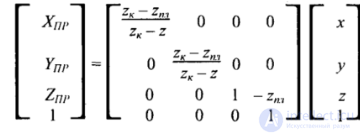
Note that here the coefficients of the matrix depend on the z coordinate (in the denominator of the fraction). This means that the coordinate transformation is nonlinear (more precisely, it is a fractional-linear transformation) and belongs to the class of projective transformations. We have obtained formulas for computing the coordinates of the projection for the case where the vanishing point of the rays lies on the z axis. Now let us consider the general case. Let us introduce a view coordinate system {X, Y, Z}, arbitrarily positioned in three-dimensional space (x, y, z). Let the vanishing point lie on the Z axis of the view coordinate system, and let the viewing direction be along the Z axis, opposite to its direction. We will assume that the transformation into view coordinates is described by a three-dimensional affine transformation. After computing the coordinates (X, Y, Z), the coordinates in the projection plane can be computed according to the formulas already considered earlier. Since the vanishing point lies on the Z axis of the view coordinates, . The sequence of coordinate transformations can be described as follows: Such a coordinate transformation makes it possible to model the placement of a camera at any point in space and to display any objects being viewed at the center of the projection plane. Fig. 2.27. Central projection of the point P0 onto the plane Z = d

Comments