Lecture
Это продолжение увлекательной статьи про статические структуры данных.
...
following should be considered already defined: the constant N is a positive integer, the number of elements in the array; the constant EMPTY is an integer, the sign is "empty" (EMPTY = -1); type - type SEQ = array [1..N] of integer; sortable sequences.
The simplest method of searching for an element that is in an unordered data set, by the value of its key, is to sequentially browse each element of the set, which continues until the desired element is found. If the entire set is viewed, but the item is not found, it means that the key being searched for is not in the set.
For a sequential search on average, (N + 1) / 2 comparisons are required. Thus, the order of the algorithm is linear - O (N).
A software illustration of a linear search in an unordered array is given in the following example, where a is the original array, key is the key that is searched; the function returns the index of the found element or EMPTY - if the element is not in the array.
  {===== Software Example 3.4 =====}
  Function LinSearch (a: SEQ; key: integer): integer;
    var i: integer;
    for i: = 1 to N do {enumeration of array elements}
      if a [i] = key then begin {key found - return index}
        LinSearch: = i;  Exit;  end;
    LinSearch: = EMPTY;  {the entire array was scanned, but the key was not found}
  end;
Another relatively simple method of accessing an element is the binary (dichotomous, binary) search method, which is performed in a well-ordered sequence of elements. Entries to the table are entered in lexicographical (character keys) or numerically (numeric keys) in ascending order. To achieve orderliness, any sorting method can be used (see 3.9).
In this method, searching for a separate entry with a specific key value resembles searching for a last name in the telephone directory. First, an entry is approximately determined in the middle of the table and its key value is analyzed. If it is too large, the value of the key corresponding to the record in the middle of the first half of the table is analyzed, and this procedure is repeated in this half until the required record is found. If the key value is too small, a key is tested that matches the record in the middle of the second half of the table, and the procedure is repeated in that half. This process continues until the required key is found or the interval in which the search is performed becomes empty.
In order to find the desired entry in the table, in the worst case, log2 (N) comparisons are required. This is significantly better than sequential search.
Программная иллюстрация бинарного поиска в упорядоченном массиве приведена в следующем примере, где a - исходный массив, key - ключ, который ищется; функция возвращает индекс найденного элемента или EMPTY - если элементт отсутствует в массиве.
 {===== Программный пример 3.5 =====}
 Function BinSearch(a : SEQ; key : integer) : integer;
 Var b, e, i : integer;
  begin
    b:=1; e:=N; { начальные значения границ }
    while b<=e do { цикл, пока интервал поиска не сузится до 0 }
    begin i:=(b+e) div 2; { середина интервала }
      if a[i]=key then
      begin BinSearch:=i; Exit; {ключ найден - возврат индекса }
      end else
        if a[i] < key then b:=i+1 { поиск в правом подинтервале }
                    else e:=i-1; { поиск в левом подинтервале }
       end; BinSearch:=EMPTY; { ключ не найден }
  end;
Trace binary search key 275 in the original sequence:
75, 151, 203, 275, 318, 489, 524, 519, 647, 777
presented in table 3.4.
| Integration | b | e | i | K [i] |
| one | one | ten | five | 318 |
| 2 | one | four | 2 | 151 |
| 3 | 3 | four | 3 | 203 |
| four | four | four | four | 275 |
Table 3.4
The binary search algorithm can be presented in a slightly different way using a recursive description. In this case, the boundary indices of the interval b and e are the parameters of the algorithm.
Recursive binary search procedure is presented in software example 3.6. To perform a search, it is necessary when calling a procedure to specify the values of its formal parameters b and e - 1 and N, respectively, where b and e are the boundary indices of the search area.
{===== Software Example 3.6 =====}
Function BinSearch (a: SEQ; key, b, e: integer): integer;
Var i: integer;
begin
if b> e then BinSearch: = EMPTY {interval width check}
else begin
i: = (b + e) div 2; {middle of interval}
if a[i]=key then BinSearch:=i {ключ найден, возврат индекса}
else if a[i] < key then { поиск в правом подинтервале }
BinSearch:=BinSearch(a,key,i+1,e)
else { поиск в левом подинтервале }
BinSearch:=BinSearch(a,key,b,i-1);
end; end;
Известно несколько модификаций алгоритма бинарного поиска, выполняемых на деревьях, которые будут рассмотрены в главе 5.
Для самого общего случая сформулируем задачу сортировки таким образом: имеется некоторое неупорядоченное входное множество ключей и должны получить выходное множество тех же ключей, упорядоченных по возрастанию или убыванию в численном или лексикографическом порядке.
Of all the programming tasks, sorting may have the richest choice of solution algorithms. Let us name some factors that influence the choice of an algorithm (besides the order of the algorithm).
one).The available memory resource: whether the input and output sets should be located in different memory areas or the output set can be formed in place of the input. In the latter case, the available memory area must be dynamically redistributed between the input and output sets during sorting; For some algorithms, this is costly, for others - with lower costs.
2). Исходная упорядоченность входного множества: во входном множестве (даже если оно сгенерировано датчиком случайных величин) могут попадаться упорядоченные участки. В предельном случае входное множество может оказаться уже упорядоченным. Одни алгоритмы не учитывают исходной упорядоченности и требуют одного и того же времени для сортировки любого (в том числе и уже упорядоченного) множества данного объема, другие выполняются тем быстрее, чем лучше упорядоченность на входе.
3). Временные характеристики операций: при определении порядка алгоритма время выполнения считается обычно пропорциональным числу сравнений ключей. Ясно, однако, что сравнение числовых ключей выполняется быстрее, чем строковых, операции пересылки, характерные для некоторых алгоритмов, выполняются тем быстрее, чем меньше объем записи, и т.п. В зависимости от характеристик записи таблицы может быть выбран алгоритм, обеспечивающий минимизацию числа тех или иных операций.
four). Сложность алгоритма является не последним соображением при его выборе. Простой алгоритм требует меньшего времени для его реализации и вероятность ошибки в реализации его меньше. При промышленном изготовлении программного продукта требования соблюдения сроков разработки и надежности продукта могут даже превалировать над требованиями эффективности функционирования.
Разнообразие алгоритмов сортировки требует некоторой их классификации. Выбран один из применяемых для классификации подходов, ориентированный прежде всего на логические характеристики применяемых алгоритмов. Согласно этому подходу любой алгоритм сортировки использует одну из следующих четырех стратегий (или их комбинацию).
one). Стратегия выборки. Из входного множества выбирается следующий по критерию упорядоченности элемент и включается в выходное множество на место, следующее по номеру.
2). Стратегия включения. Из входного множества выбирается следующий по номеру элемент и включается в выходное множество на то место, которое он должен занимать в соответствии с критерием упорядоченности.
3). Стратегия распределения. Входное множество разбивается на ряд подмножеств (возможно, меньшего объема) и сортировка ведется внутри каждого такого подмножества.
four). Стратегия слияния. Выходное множество получается путем слияния маленьких упорядоченных подмножеств.
Далее приводится обзор (далеко не полный) методов сортировки, сгруппированных по стратегиям, применяемым в их алгоритмах. Все алгоритмы рассмотрены для случая упорядочения по возрастанию ключей.
Сортировка простой выборкой.
Данный метод реализует практически "дословно" сформулированную выше стратегию выборки. Порядок алгоритма простой выборки - O(N^2). Количество пересылок - N.
Алгоритм сортировки простой выборкой иллюстрируется программным примером 3.7.
В программной реализации алгоритма возникает проблема значения ключа "пусто". Довольно часто программисты используют в качестве такового некоторое заведомо отсутствующее во входной последовательности значение ключа, например, максимальное из теоретически возможных значений. Другой, более строгий подход - создание отдельного вектора, каждый элемент которого имеет логический тип и отражает состояние соответствующего элемента входного множества ("истина" - "непусто", "ложь" - "пусто"). Именно такой подход реализован в нашем программном примере. Роль входной последовательности здесь выполняет параметр a, роль выходной - параметр b, роль вектора состояний - массив c. Алгоритм несколько усложняется за счет того, что для установки начального значения при поиске минимума приходится отбрасывать уже "пустые" элементы.
 {===== Software Example 3.7 =====}
 Procedure Sort (a: SEQ; var b: SEQ);
 Var i, j, m: integer;
      c: array [1..N] of boolean; {state of elements in set}
  begin
   for i: = 1 to N do c [i]: = true; {reset marks}
   for i: = 1 to N do {search for the 1st unselected email. in the set}
    begin j: = 1;
          while not c [j] do j: = j + 1;
          m: = j; {search for the minimum element a}
     for j: = 2 to N do
       if c [j] and (a [j]
     b [i]: = a [m]; {write to output set}
     c [m]: = false; {in the input set - "empty"}
  end;  end;
Exchange sorting by simple sampling.
A simple sampling algorithm, however, is rarely used in the version in which it is described above. It is much more often used its so-called exchange option. With exchange sorting, the input and output sets are located in the same memory area; output - at the beginning of the area, input - in the rest of it. In the initial state, the input set occupies the entire region, and the output set is empty. As the sorting is performed, the input set narrows and the output set expands.
Exchange sorting by simple sampling is shown in software example 3.8. The procedure has only one parameter - the array to be sorted.
 {===== Software Example 3.8 =====}
 Procedure Sort (var a: SEQ);
 Var x, i, j, m: integer;
  begin
   for i: = 1 to N-1 do {enumerating the elements of the output set}
   {input set - [i: N]; output - [1: i-1]}
     begin m: = i;
      for j: = i + 1 to N do {search for the minimum in the input set}
        if (a [j]
      {exchange of the 1st element in. sets with minimal}
      if i <> m then begin
        x: = a [i]; a [i]: = a [m]; a [m]: = x;
  end; end;  end;
The trace results of the software example 3.8 are presented in table 3.5. The colon shows the boundary between the input and output sets.
| Step | Array content a |
| Original | : 242 447 286 708_24_11 192 860 937 561 |
| one | _11: 447 286 708_ 24 242 192 860 937 561 |
| 2 | _11_24: 286 708 447 242 192 860 937 561 |
| 3 | _11_24 192: 708 447 242 286 860 937 561 |
| four | _11_24 192 242: 447 708 286 860 937 561 |
| five | _11_24 192 242 286: 708 447 860 937 561 |
| 6 | _11_24 192 242 286 447: 708 860 937 561 |
| 7 | _11_24 192 242 286 447 561: 860 937 708 |
| eight | _11_24 192 242 286 447 561 708: 937 860 |
| 9 | _11_24 192 242 286 447 561 708 860: 937 |
| Result | _11_24 192 242 286 447 561 708 860 937: |
Таблица 3.5
Очевидно, что обменный вариант обеспечивает экономию памяти. Очевидно также, что здесь не возникает проблемы "пустого" значения. Общее число сравнений уменьшается вдвое - N*(N-1)/2, но порядок алгоритма остается степенным - O(n^2). Количество перестановок N-1, но перестановка, по-видимому, вдвое более времяемкая операция, чем пересылка в предыдущем алгоритме.
Довольно простая модификация обменной сортировки выборкой предусматривает поиск в одном цикле просмотра входного множества сразу и минимума, и максимума и обмен их с первым и с последним элементами множества соответственно. Хотя итоговое количество сравнений и пересылок в этой модификации не уменьшается, достигается экономия на количестве итераций внешнего цикла.
Приведенные выше алгоритмы сортировки выборкой практически нечувствительны к исходной упорядоченности. В любом случае поиск минимума требует полного просмотра входного множества. В обменном варианте исходная упорядоченность может дать некоторую экономию на перестановках для случаев, когда минимальный элемент найден на первом месте во входном множестве.
Пузырьковая сортировка.
Входное множество просматривается, при этом попарно сравниваются соседние элементы множества. Если порядок их следования не соответствует заданному критерию упорядоченности, то элементы меняются местами. В результате одного та- кого просмотра при сортировке по возрастанию элемент с самым большим значением ключа переместится ("всплывет") на последнее место в множестве. При следующем проходе на свое место "всплывет" второй по величине ключа элемент и т.д. Для постановки на свои места N элементов следует сделать N-1 проходов. Выходное множество, таким образом, формируется в конце сортируемой последовательности, при каждом следующем проходе его объем увеличивается на 1, а объем входного множества уменьшается на 1.
Порядок пузырьковой сортировки - O(N^2). Среднее число сравнений - N*(N-1)/2 и таково же среднее число перестановок, что значительно хуже, чем для обменной сортировки простым выбором. Однако, то обстоятельство, что здесь всегда сравниваются и перемещаются только соседние элементы, делает пузырьковую сортировку удобной для обработки связных списков. Перестановка в связных списках также получается более экономной.
Еще одно достоинство пузырьковой сортировки заключается в том, что при незначительных модификациях ее можно сделать чувствительной к исходной упорядоченности входного множества. Рассмотрим некоторые их таких модификаций.
Во-первых, можно ввести некоторую логическую переменную, которая будет сбрасываться в false перед началом каждого прохода и устанавливаться в true при любой перестановке. Если по окончании прохода значение этой переменной останется false, это означает, что менять местами больше нечего, сортировка закончена. При такой модификации поступление на вход алгоритма уже упорядоченного множества потребует только одного просмотра.
Во-вторых, может быть учтено то обстоятельство, что за один просмотр входного множества на свое место могут "всплыть" не один, а два и более элементов. Это легко учесть, запоминая в каждом просмотре позицию последней перестановки и установки этой позиции в качестве границы между множествами для следующего просмотра. Именно эта модификация реализована в программной иллюстрации пузырьковой сортировке в примере 3.9. Переменная nn в каждом проходе устанавливает верхнюю границу входного множества. В переменной x запоминается позиция перестановок и в конце просмотра последнее запомненное значение вносится в nn. Сортировка будет закончена, когда верхняя граница входного множества станет равной 1.
 {===== Программный пример 3.9 =====}
 Procedure Sort( var a : seq);
 Var nn, i, x : integer;
  begin
   nn:=N; { граница входного множества }
   repeat x:=1; { признак перестановок }
     for i:=2 to nn do { перебор входного множества }
     if a[i-1] > a[i] then begin { сравнение соседних эл-в }
       x:=a[i-1]; a[i-1]:=a[i]; a[i]:=x; { перестановка }
       x:=i-1; { запоминание позиции }
      end; nn:=x; { сдвиг границы }
   until (nn=1); {цикл пока вых. множество не захватит весь мас.}
  end;
Результаты трассировки программного примера 3.9 представлены в таблице 3.6.
| Step | nn | Содержимое массива а |
| Исходный | ten | 717 473 313 160 949 764_34 467 757 800: |
| one | 9 | 473 313 160 717 764_34 467 757 800:949 |
| 2 | 7 | 313 160 473 717_34 467 757:764 800 949 |
| 3 | five | 160 313 473_34 467:717 757 764 800 949 |
| four | four | 160 313_34 467:473 717 757 764 800 949 |
| five | 2 | 160_34:313 467 473 717 757 764 800 949 |
| 6 | one | _34:160 313 467 473 717 757 764 800 949 |
| Result | : 34 160 313 467 473 717 757 764 800 949 |
Таблица 3.6
Еще одна модификация пузырьковой сортировки носит название шейкер-сортировки. Суть ее состоит в том, что направления просмотров чередуются: за просмотром от начала к концу следует просмотр от конца к началу входного множества. При просмотре в прямом направлении запись с самым большим ключом ставится на свое место в последовательности, при просмотре в обратном направлении - запись с самым маленьким. Этот алгоритм весьма эффективен для задач восстановления упорядоченности, когда исходная последовательность уже была упорядочена, но подверглась не очень значительным изменениям. Упорядоченность в последовательности с одиночным изменением будет гарантированно восстановлена всего за два прохода.
Сортировка Шелла.
Это еще одна модификация пузырьковой сортировки. Суть ее состоит в том, что здесь выполняется сравнение ключей, отстоящих один от другого на некотором расстоянии d. Исходный размер d обычно выбирается соизмеримым с половиной общего размера сортируемой последовательности. Выполняется пузырьковая сортировка с интервалом сравнения d. Затем величина d уменьшается вдвое и вновь выполняется пузырьковая сортировка, далее d уменьшается еще вдвое и т.д. Последняя пузырьковая сортировка выполняется при d=1. Качественный порядок сортировки Шелла остается O(N^2), среднее же число сравнений, определенное эмпирическим путем - log2(N)^2*N. Ускорение достигается за счет того, что выяв- ленные "не на месте" элементы при d>1, быстрее "всплывают" на свои места.
Пример 3.10 иллюстрирует сортировку Шелла.
 {===== Программный пример 3.10 =====}
 Procedure Sort (var a: seq);
 Var d, i, t: integer; k: boolean; {sign of permutation}
 begin d: = N div 2; {initial interval value}
   while d> 0 do {cycle with decreasing interval to 1}
     begin k: = true; {bubble sort with d interval}
     while k do {cycle while there are permutations}
       begin k: = false;  i: = 1;
       for i: = 1 to Nd do {comparison of emails on the interval d}
          begin if a [i]> a [i + d] then begin
           t: = a [i]; a [i]: = a [i + d]; a [i + d]: = t; {permutation}
           k: = true; {sign of permutation}
            end;{if ...} end; {for ...} end; {while k}
      d: = d div 2; {decrease interval}
      end; {while d> 0} end;
The trace results of the software example 3.10 are presented in table 3.7.
| Step | d | Array content a |
| Original | 76 22_ 4 17 13 49_ 4 18 32 40 96 57 77 20_ 1 52 | |
| one | eight | 32 22_ 4 17 13 20_ 1 18 76 40 96 57 77 49_ 4 52 |
| 2 | eight | 32 22_ 4 17 13 20_ 1 18 76 40 96 57 77 49_ 4 52 |
| 3 | four | 13 20_ 1 17 32 22_ 4 18 76 40_ 4 52 77 49 96 57 |
| four | four | 13 20_ 1 17 32 22_ 4 18 76 40_ 4 52 77 49 96 57 |
| five | 2 | 13 20_ 1 17 32 22_ 4 18 76 40_ 4 52 77 49 96 57 |
| 6 | 2 | 13 20_ 1 17 32 22_ 4 18 76 40_ 4 52 77 49 96 57 |
| 7 | 2 | _1 17_ 4 18_ 4 20 13 22 32 40 76 49 77 52 96 57 |
| eight | 2 | _1 17_ 4 18_ 4 20 13 22 32 40 76 49 77 52 96 57 |
| 9 | one | _1_ 4 17_ 4 18 13 20 22 32 40 49 76 52 77 57 96 |
| ten | one | _1_ 4_ 4 17 13 18 20 22 32 40 49 52 76 57 77 96 |
| eleven | one | _1_ 4_ 4 13 17 18 20 22 32 40 49 52 57 76 77 96 |
| 12 | one | _1_ 4_ 4 13 17 18 20 22 32 40 49 52 57 76 77 96 |
| Result | _1_ 4_ 4 13 17 18 20 22 32 40 49 52 57 76 77 96 |
Таблица 3.7
Сортировка простыми вставками.
Этот метод - "дословная" реализации стратегии включения. Порядок алгоритма сортировки простыми вставками - O(N^2), если учитывать только операции сравнения. Но сортировка требует еще и в среднем N^2/4 перемещений, что де- лает ее в таком варианте значительно менее эффективной, чем сортировка выборкой.
Алгоритм сортировки простыми вставками иллюстрируется программным примером 3.11.
 {===== Программный пример 3.11 =====}
 Procedure Sort(a : Seq; var b : Seq);
   Var i, j, k : integer;
    begin
     for i:=1 to N do begin { перебор входного массива }
       { поиск места для a[i] в выходном массиве }
        j: = 1; while (j < i) and (b[j] <= a[i]) do j:=j+1;
       { освобождение места для нового эл-та }
       for k:=i downto j+1 do b[k]:=b[k-1];
       b[j]:=a[i]; { запись в выходной массив }
        end;  end;
Эффективность алгоритма может быть несколько улучшена при применении не линейного, а дихотомического поиска. Однако, следует иметь в виду, что такое увеличение эффективности может быть достигнуто лишь на множествах значительного по количеству элементов объема. Because алгоритм требует большого числа пересылок, при значительном объеме одной записи эффективность может определяться не количеством операций сравнения, а количеством пересылок.
Реализация алгоритма обменной сортировки простыми вставками отличается от базового алгоритма только тем, что входное и выходное множество разделяют одну область памяти.
Пузырьковая сортировка вставками.
Это модификация обменного варианта сортировки. В этом методе входное и выходное множества находятся в одной последовательности, причем выходное - в начальной ее части. В исходном состоянии можно считать, что первый элемент последовательности уже принадлежит упорядоченному выходному множеству, остальная часть последовательности - неупорядоченное входное. Первый элемент входного множества примыкает к концу выходного множества. На каждом шаге сортировки происходит перераспределение последовательности: выходное множество увеличивается на один элемент, а входное - уменьшается. Это происходит за счет того, что первый элемент входного множества теперь считается последним элементом выходного. Затем выполняется просмотр выходного множества от конца к началу с перестановкой соседних элементов, которые не соответствуют критерию упорядоченности. Просмотр прекращается, когда прекращаются перестановки. Это приводит к тому, что последний элемент выходного множества "выплывает" на свое место в множестве. Поскольку при этом перестановка приводит к сдвигу нового в выходном множестве элемента на одну позицию влево, нет смысла всякий раз производить полный обмен между соседними элементами - достаточно сдвигать старый элемент вправо, а новый элемент записать в выходное множество, когда его место будет установлено. Именно так и построен программный пример пузырьковой сортировки вставками - 3.12.
 {===== Программный пример 3.12 =====}
 Procedure Sort (var a : Seq);
 Var i, j, k, t : integer;
  begin
   for i:=2 to N do begin { перебор входного массива }
   {*** вх.множество - [i..N], вых.множество - [1..i] }
     t:=a[i]; { запоминается значение нового эл-та }
     j:=i-1; {поиск места для эл-та в вых. множестве со сдвигом}
       { цикл закончится при достижении начала или, когда
         будет встречен эл-т, меньший нового }
       while (j >= 1) and (a[j] > t) do begin
         a[j+1]:=a[j]; { все эл-ты, большие нового сдвигаются }
          j: = j-1; { цикл от конца к началу выходного множества }
          end;
       a[j+1]:=t; { новый эл-т ставится на свое место }
        end;
  end;
Результаты трассировки программного примера 3.11 представлены в таблице 3.8.
| Step | Содержимое массива a |
| Исходный | 48:43 90 39_ 9 56 40 41 75 72 |
| one | 43 48:90 39_ 9 56 40 41 75 72 |
| 2 | 43 48 90:39_ 9 56 40 41 75 72 |
| 3 | 39 43 48 90:_9 56 40 41 75 72 |
| four | _9 39 43 48 90:56 40 41 75 72 |
| five | _9 39 43 48 56 90:40 41 75 72 |
| 6 | _9 39 40 43 48 56 90:41 75 72 |
| 7 | _9 39 40 41 43 48 56 90:75 72 |
| eight | _9 39 40 41 43 48 56 75 90:72 |
| Result | _9 39 40 41 43 48 56 72 75 90: |
Таблица 3.8
Хотя обменные алгоритмы стратегии включения и позволяют сократить число сравнений при наличии некоторой исходной упорядоченности входного множества, значительное число пересылок существенно снижает эффективность этих алгоритмов. Поэтому алгоритмы включения целесообразно применять к связным структурам данных, когда операция перестановки элементов структуры требует не пересылки данных в памяти, а выполняется способом коррекции указателей (см. главу 5).
Еще одна группа включающих алгоритмов сортировки использует структуру дерева. Мы рекомендуем читателю повторно вернуться к рассмотрению этих алгоритмов после ознакомления с главой 6.
Сортировка упорядоченным двоичным деревом.
Алгоритм складывается из построения упорядоченного двоичного дерева и последующего его обхода. Если нет необходимости в построении всего линейного упорядоченного списка значений, то нет необходимости и в обходе дерева, в этом случае применяется поиск в упорядоченном двоичном дереве. Алгоритмы работы с упорядоченными двоичными деревьями подробно рассмотрены в главе 6. Отметим, что порядок алгоритма - O(N*log2(N)), но в конкретных случаях все зависит от упорядоченности исходной последовательности, который влияет на степень сбалансированности дерева и в конечном счете - на эффективность поиска.
Турнирная сортировка.
Этот метод сортировки получил свое название из-за сходства с кубковой системой проведения спортивных соревнований: участники соревнований разбиваются на пары, в которых разыгрывается первый тур; из победителей первого тура составляются пары для розыгрыша второго тура и т.д. Алгоритм сортировки состоит из двух этапов. На первом этапе строится дерево: аналогичное схеме розыгрыша кубка.
For example, for a sequence of numbers a:
16 21 8 14 26 94 30 1
such a tree will have the appearance of a pyramid, shown in Figure 3.13.
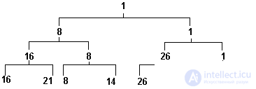
Fig.3.13. Tournament sorting pyramid
Example 3.12 provides a software illustration of the tournament sorting algorithm. She needs some explanations. Pyramid construction is performed by the Create_Heap function. The pyramid is built from the bottom to the top. The elements that make up each level are linked into a linear list, so every node in the tree, besides the usual pointers to descendants, left and right, also contains a pointer to “brother” —next. When working with each level, the pointer contains the starting address of the list of elements in this level. In the first phase, a linear list is constructed for the lower level of the pyramid, into the elements of which the keys from the initial sequence are entered. The next while loop in each of its iterations adds the next level of the pyramid. The condition for the completion of this cycle is to obtain a list consisting of a single element, that is, the apex of the pyramid. The construction of the next level consists in a pair-wise iteration of the elements of the list constituting the previous (lower) level. The smallest key value from each pair is transferred to the new level.
The next stage consists in sampling values from the pyramid and forming an ordered sequence from them (the Heap_Sort procedure and the Competit function). In each iteration of the Heap_Sort procedure loop, a value is selected from the top of the pyramid — this is the smallest key value in the pyramid. At the same time, the node-node is released, and all nodes occupied by the selected value at lower levels of the pyramid are also released. For the vacated nodes, a contest between their descendants is organized (from the bottom up). So, for the pyramid, the initial state of which was shown in Fig. 3., when sampling the first three keys (1, 8, 14), the pyramid will consistently take the form shown in Fig. 3.14 (x marks empty spaces in the pyramid).
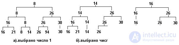
Fig.3.14. Pyramid after consecutive samples
The procedure Heap_Sort gets the input parameter ph - a pointer to the top of the pyramid. and forms the output parameter a - an ordered array of numbers. The entire Heap_Sort procedure consists of a loop, in each iteration of which the value from the vertex is transferred to array a, and then the Competit function is called, which provides for the reorganization of the pyramid due to the removal of the value from the vertex.
The Competet function is recursive, its parameter is a pointer to the top of the subtree to be reorganized. In the first phase of the function, it is established whether the node constituting the vertex of the specified subtree has a descendant whose data value matches the data value at the vertex. If there is such a descendant, the Competit function calls itself to reorganize the subtree whose top is the detected descendant. After reorganization, the child's address in the node is replaced with the address that returned the recursive call to Competit. If after the reorganization it turns out that the node has no descendants (or it had no descendants from the very beginning), then the node is destroyed and the function returns a null pointer. If the node still has descendants, then the value of the data from the descendant in which this value is the smallest is entered in the data field of the node, and the function returns the previous address of the node.
  {===== Software Example 3.12 =====}
  {Tournament sorting}
  type nptr = ^ node;  {pointer to node}
      node = record {tree node}
        key: integer;  {data}
        left, right: nptr;  {pointers to descendants}
        next: nptr;  {pointer to "brother"}
        end;
  {Creating a tree - the function returns a pointer to the top
                      created tree}
  Function Heap_Create (a: Seq): nptr;
    var i: integer;
        ph2: nptr;  {address of the beginning of the list of level}
        p1: nptr;  {address of new item}
        p2: nptr;  {address of the previous element}
        pp1, pp2: nptr;  {addresses of the competing pair}
    begin
    {Phase 1 - building the lowest level of the pyramid}
    ph2: = nil;
    for i: = 1 to n do begin
      New (p1);  {memory allocation for new el-ta}
      p1 ^ .key: = a [i];  {write data from array}
      p1 ^ .left: = nil;  p1 ^ .right: = nil;  {no descendants}
      {linking to a linear list by level}
      if ph2 = nil then ph2: = p1 else p2 ^ .next: = p1;
      p2: = p1;
      end;  {for}
    p1 ^ .next: = nil;
    {Phase 2 - building other levels}
    while ph2 ^ .next <> nil do begin {cycle to the top of the pyramid}
      pp1: = ph2;  ph2: = nil;  {start new level}
      while pp1 <> nil do begin {cycle on the next level}
        pp2: = pp1 ^ .next;
        New (p1);
        {addresses of descendants from the previous level}
        p1 ^ .left: = pp1;  p1 ^ .right: = pp2;
        p1 ^ .next: = nil;
        {linking to a linear list by level}
        if ph2 = nil then ph2: = p1 else p2 ^ .next: = p1;
        p2: = p1;
        {data contention for reaching the level}
        if (pp2 = nil) or (pp2 ^ .key> pp1 ^ .key) then p1 ^ .key: = pp1 ^ .key
        else p1 ^ .key: = pp2 ^ .key;
        {go to the next couple}
        if pp2 <> nil then pp1: = pp2 ^ .next else pp1: = nil;
        end;  {while pp1 <> nil}
      end;  {while ph2 ^ .next <> nil}
    Heap_Create: = ph2;
  end;
    {Reorganize subtree - function returns
      pointer to the top of the reorganized tree}
  Function Competit (ph: nptr): nptr;
    begin
    {determination of descendants, choice of descendant for
      reorganization, reorganization of it}
    if (ph ^ .left <> nil) and (ph ^ .left ^ .key = ph ^ .key) then
      ph ^ .left: = Competit (ph ^ .left)
    else if (ph ^ .right <> nil) then
      ph ^ .right: = Competit (ph ^ .right);
    if (ph ^ .left = nil) and (ph ^ .right = nil) then begin
      {empty empty node}
      Dispose (ph);  ph: = nil;
      end;
    else
      {contention of descendants}
      if (ph ^ .left = nil) or
      ((ph ^ .right <> nil) and (ph ^ .left ^ .key> ph ^ .right ^ .key)) then
         ph ^ .key: = ph ^ .right ^ .key
       else ph ^ .key: = ph ^ .left ^ .key;
    Competit: = ph;
  end;
  {Sort}
  Procedure Heap_Sort (var a: Seq);
    var ph: nptr;  {address of the top of the tree}
        i: integer;
    begin
    ph: = Heap_Create (a);  {making a tree}
    {wood sampling}
    for i: = 1 to N do begin
      {transfer data from vertex to array}
      a [i]: = ph ^ .key;
      {reorganize the tree}
      ph: = Competit (ph);
      end;
  end;
Tree construction requires N-1 comparisons, sampling - N * log2 (N) comparisons. The order of the algorithm is thus O (N * log2 (N)). The complexity of operations on connected data structures, however, is significantly higher than on static structures. In addition, the algorithm is uneconomical in terms of memory: duplication of data at different levels of the pyramid leads to the fact that the working area of memory contains approximately 2 * N nodes.
Sort by partially ordered tree.
In the binary tree that is built in this sorting method for each node, the following statement is true: the key value written in the node is less than the keys of its descendants. For a fully ordered tree, there are requirements for the relationship between keys of descendants. There are no such requirements for this tree, therefore such a tree is called partially ordered. In addition, our tree must be absolutely balanced. This means not only that the lengths of paths to any two leaves differ by no more than 1, but also that when adding a new element to the tree, the left branch / sub-branch is always preferred, as long as it does not disturb the balance. In more detail, trees are discussed in Chapter 6.
For example, a sequence of numbers:
3 20 12 58 35 30 32 28
will be presented in the form of a tree shown in Figure 3.15.
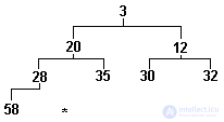
Fig.3.15. Partially ordered tree
The representation of the tree in the form of a pyramid clearly shows us that for such a tree, we can introduce the concepts of "beginning" and "end". The beginning, naturally, will be considered the top of the pyramid, and the end - the leftmost element in the lowest row (in Figure 3.15 it is 58).
To sort by this method, two operations must be defined: inserting a new element into the tree and selecting the minimum element from the tree; moreover, the performance of any of these operations should not violate the partial ordering of the tree formulated above, nor its balance.
The insertion algorithm is as follows. A new element is inserted into the first free space at the end of the tree (in Figure 3.15, this place is indicated by the symbol "*"). If the key of the inserted element is smaller than the key of its ancestor, then the ancestor and the inserted element are swapped. The key of the inserted element is now compared with the key of its ancestor in a new place, etc. Comparisons end when the key of the new element is greater than the key of the ancestor or when the new element pops into the top of the pyramid. The pyramid, shown in Figure 3.15, is constructed by successively including numbers from the series listed in it. If we include in it, for example, the number 16, then the pyramid will take the form shown in Figure 3.16. (The "*" symbol denotes elements moved during this operation.)
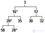
Fig.3.16. Partially ordered tree, element inclusion
The procedure for selecting an item is somewhat more complicated. Obviously, the minimal element is at the vertex. After sampling, the competition between the descendants is arranged for the vacated space, and the descendant with the lowest key value moves to the vertex. For the vacant place of the mixed descendant, its descendants compete, etc., until the free space reaches the pyramid sheet. The state of our tree after sampling the minimum number (3) from it is shown in Figure 3.17. A.
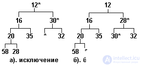
Fig.3.17. Partially ordered tree, item elimination
The order of the tree has been restored, but the condition for its balance has been violated, since the free space is not at the end of the tree. To restore balance, the last element of the tree is transferred to the vacant space, and then "pops up" by the same algorithm that was used when inserting. The result of this balancing is shown in Figure 3.17.b.
Before describing a software example illustrating sorting by a partially ordered tree — Example 3.13, let us draw the reader’s attention to the way the tree is represented in memory in it. This is a way of representing binary trees in static memory (in a one-dimensional array), which can be applied in other tasks. Elements of the tree are located in the adjacent memory slots by levels. The very first slot of the allocated memory occupies the top. The next 2 slots are second level elements, the next 4 slots are third, and so on. The tree from Figure 3.17.b, for example, will be linearized in this way:
12 16 28 20 35 30 32 58
In this view, there is no need to store pointers as part of the tree node, since the addresses of the children can be calculated. For a node represented by an array element with index i, the indices of its left and right descendants are 2 * i and 2 * i + 1, respectively. For a node with index i, its ancestor index will be i div 2.
After all of the above, the algorithm of software example 3.13 does not need any special explanations. We explain only the structure of the example. The example is designed as a complete program module, which will be used in the following example. The tree itself is represented in the tree array, the variable nt is the index of the first free element in the array. Module input points:
In addition, the module defines internal program units:
  {===== Software Example 3.13 =====}
  {Sort by partially ordered tree}
  Unit SortTree;
  Interface
  Procedure InitSt;
  Function CheckST (var a: integer): integer;
  Function DeleteST (var a: integer): boolean;
  Function InsertST (a: integer): boolean;
  Implementation
  Const NN = 16;
  var tr: array [1..NN] of integer;  { tree }
      nt: integer;  {index of the last item in the tree}
  {** Ascent from place with index l **}
  Procedure Up (l: integer);
    var h: integer;  {l is the node index, h is the index of its ancestor}
        x: integer;
    begin
    h: = l div 2;  {ancestor index}
    while h> 0 do {before the beginning of the tree}
      if tr [l]
If you use sorting by a partially ordered tree to order an already prepared sequence of size N, then you need to do the insertion N times, and then N times the selection. The order of the algorithm is O (N * log2 (N)), but the average value of the number of comparisons is about 3 times greater than for tournament sorting. But sorting a partially ordered tree has one significant advantage over all other algorithms. The fact is that this is the most convenient algorithm for "sorting on-line", when the sorting sequence is not fixed before the start of sorting, but changes during work and inserts alternate with samples. Each change (adding / deleting an element) of a sorted sequence will require no more than 2 * log2 (N) comparisons and permutations, while other algorithms will require re-ordering of the entire sequence "by the complete program" with a single change.
A typical task that requires this sorting occurs when data is sorted on external memory (files). The first stage of such sorting is the formation of the ordered sequences of the maximum possible length from the file data with a limited amount of RAM. The following program example (Example 3.14) shows the solution to this problem.
The sequence of numbers written in the input file is read elementwise and the numbers are included in the tree as they are read. When the tree is full, the next number read from the file is compared with the last number output to the output file. If the read number is not less than the last displayed, but less than the number located at the top of the tree, then the read number is output to the output file. If the read number is not less than the last output, and not less than the number at the top of the tree, then the number selected from the tree is output to the output file, and the read number is entered in the tree. Finally, if the read number is less than the last derived one, then the entire contents of the tree is selected and output element by element, and the formation of a new sequence begins with an entry of the read number into an empty tree.
  {===== Software Example 3.14 =====}
  {Formation of sorted sequences in the file}
  Uses SortTree;
  var x: integar;  {read number}
      y: integer;  {number at the top of the tree}
      old: integer;  {last number displayed}
      inp: text;  {input file}
      out: text;  {output file}
      bf: boolean;  {flag to start outputting a sequence}
      bx: boolean;  {working variable}
  begin
  Assign (inp, 'STX.INP');  Reset (inp);
  Assign (out, 'STX.OUT');  Rewrite (out);
  InitST;  {sorting initialization}
  bf: = false;  {sequence output not started yet}
  while not Eof (inp) do begin
    ReadLn (inp, x);  {read number from file}
    {if there is free space in the tree - include it in the tree}
    if CheckST (y) <= 1 then bx: = InsertST (x)
продолжение следует...
Часть 1 3. STATIC DATA STRUCTURE
Часть 2 3.8. Операции логического уровня над статическими структурами. Sorting - 3.
Часть 3 3.8.3. Sort by distribution. - 3. STATIC DATA STRUCTURE

Comments
To leave a comment
Structures and data processing algorithms.
Terms: Structures and data processing algorithms.