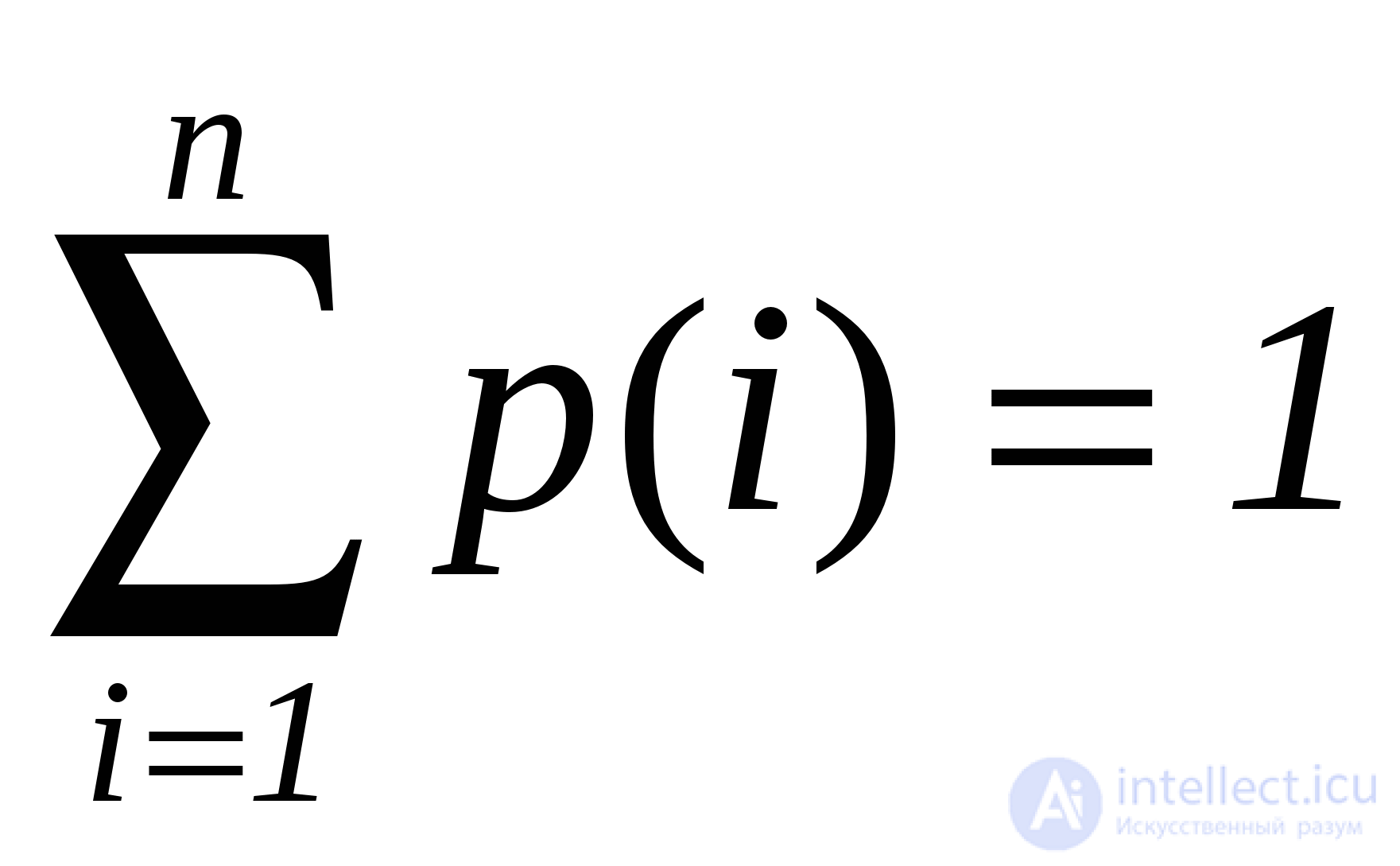
You can always talk about a certain value of the probability of finding one or another element in the table. We assume that this element exists in the table. Then the entire lookup table can be represented as a system with discrete states, and the probability of finding the desired element there is the probability of the
p (i) i -th state of the system.

The number of comparisons when searching in the table presented as a discrete system is the mathematical expectation of the value of a discrete random variable determined by the probabilities of states and numbers of states of the system.
Z = Q = 1p (1) + 2p (2) + 3p (3) + ... + np (n) It is desirable that
p (1) ³ p (2) ³ p (3) ³ … ³ p (n). This minimizes the number of comparisons, i.e. increases efficiency. Since a consecutive search begins with the first element, then the element to which it is most often addressed (with the highest probability of search) must be put on this place.
The two most commonly used methods are the autonomous reordering of lookup tables. Consider them on the example of simply linked lists.
5.5.1 Reordering the lookup table by swapping the found item to the top of the list
The essence of this method is that a list item with a key equal to a given one becomes the first item in the list, and all the others are shifted.

This algorithm is applicable to both lists and arrays. However, it is not recommended to use it for arrays, since it takes much longer to rearrange the elements of an array than to rearrange the pointers.
The reordering algorithm to the top of the list:
Pseudocode:
q = nil
p = table
while (p <> nil) do
if key = k (p) then
if q = nil then 'no need permutation'
search = p
return
endif
nxt (q) = nxt (p)
nxt (p) = table
table = p
search = p
return
endif
q = p
p = nxt (p)
endwhile
search = nil
return |
Pascal:
q: = nil;
p: = table;
while (p <> nil) do
begin
if key = p ^ .k then
begin
if q = nil
then 'swap is not needed'
search: = p;
exit;
end;
q ^ .nxt: = p ^ .nxt;
p ^ .nxt: = table;
table: = p;
exit;
end;
q: = p;
p: = p ^ .nxt;
end;
search: = nil;
exit; |
5.5.2. Transposition method
In this method, the found element is rearranged by one element to the head of the list. And if this element is often accessed, then moving to the head of the list, it will soon be in the first place.

p - working pointer
q - auxiliary pointer, one step behind p
s - auxiliary pointer, two steps behind q
Algorithm of transposition method:
Pseudocode:
s = nil
q = nil
p = table
while (p <> nil) do
if key = k (p) then
'found transposable
if q = nil then
'no need to rearrange
search = p
return
endif
nxt (q) = nxt (p)
nxt (p) = q
if s = nil then
table = p
else nxt (s) = p
endif
search = p
return
endif
endwhile
search = nil
return |
Pascal:
s: = nil;
q: = nil;
p: = table;
while (p <> nil) do
begin
if key = p ^ .k then
'found transposable
begin
if q = nil then
begin
'not rearranged
to search: = p;
exit;
end;
q ^ .nxt: = p ^ .nxt;
p ^ .nxt: = q;
if s = nil then
table: = p;
else
begin
s ^ .nxt: = p;
end;
search: = p;
exit;
end;
end;
search: = nil;
exit; |
This method is useful when searching not only in lists, but also in arrays (since only two adjacent elements change).
5.5.3. Optimal Search Tree
If the extracted elements have formed some constant set, then it may be beneficial to customize the binary search tree for more efficient subsequent search.
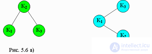
Consider the binary search trees shown in Figures a and b. Both trees contain three elements -
k1, k2, k3, where
k1 <k2 <k3 . The search for element
k3 requires two comparisons for Figure 5.6 a), and only one for Figure 5.6 b).
The number of key comparisons that need to be made to extract some record is equal to the level of this record in the binary search tree plus 1.
Let's pretend that:
p 1 - the probability that the argument of the search
key = K1 p2 is the probability that the search argument is
key = k2 p3 is the probability that the search argument is
key = k3 q 0 is the probability that
key <к1 q 1 - the probability that
k2> key > k1 q 2 - the probability that
k3> key > k2 q 3 - the probability that
key > k3 C 1 is the number of comparisons in the first tree of Figure 5.6 a)
C 2 - the number of comparisons in the second tree of Figure 5.6 b)

Then
× p1 + × p2 + × p3 + × q0 + × q1 + × q2 + × q3 = 1 The expected number of comparisons in some search is the sum of the products of the probability that a given argument has a given value, the number of comparisons needed to extract this value, where the sum is taken over all possible values of the search argument. therefore
C1 = 2 × p1 + 1 × p2 + 2 × p3 + 2 × q0 + 2 × q1 + 2 × q2 + 2 × q3 C2 = 2 × p1 + 3 × p2 + 1 × p3 + 2 × q0 + 3 × q1 + 3 × q2 + 1 × q3 This expected number of comparisons can be used as a measure of how well a particular binary search tree is suitable for a given set of keys and a given set of probabilities. So, for the probabilities given below on the left, the tree from a) is more efficient, and for the probabilities given on the right, the tree from b) is more efficient:
P1 = 0.1 P1 = 0.1 P2 = 0.3 P2 = 0.1 P3 = 0.1 P3 = 0.3 q0 = 0.1 q0 = 0.1 q1 = 0.2 q1 = 0.1 q2 = 0.1 q2 = 0.1 q3 = 0.1 q3 = 0.2 C1 = 1.7 C1 = 1.9 C2 = 2.4 C2 = 1.8 A binary search tree that minimizes the expected number of comparisons of a given set of keys and probabilities is called optimal. Although the tree creation algorithm can be very time consuming, the tree it creates will work effectively in all subsequent searches. Unfortunately, however, the probabilities of search arguments are rarely known in advance.


Comments
To leave a comment
Structures and data processing algorithms.
Terms: Structures and data processing algorithms.