
Lecture
A parallel connection of sections of an electric circuit is a connection in which all sections of the circuit are attached to the same pair of nodes, i.e., are subjected to the same voltage (Fig. 3.8). The currents of parallel-connected sections are inversely proportional to the resistances of those sections.
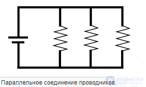
The current in the unbranched part of the circuit is equal to the sum of the currents in the individual parallel-connected conductors: 
The voltage across sections AB of the circuit and across the ends of all parallel-connected conductors is one and the same: 
When resistors are connected in parallel, the quantities inversely proportional to resistance are added (that is, the total conductance  is made up of the conductances of each resistor
  )
)
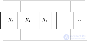
If the circuit can be broken down into nested sub-blocks connected to each other in series or in parallel, the resistance of each sub-block is calculated first, then each sub-block is replaced by its equivalent resistance; in this way the total (sought) resistance is found.
For two parallel-connected resistors, their total resistance is equal to: 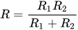 .
.
If  , then the total resistance is equal to:
  .
.
When resistors are connected in parallel, their total resistance will be less than the smallest of the resistances.

 .
.

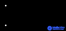
The circuit is closed when at least one of the switches is closed. (analogous to the logical OR operation).
When resistances R1, R2 and R3 are connected in parallel, the load currents are respectively equal to
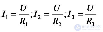
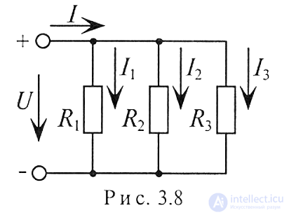
Using Kirchhoff's first law, the current I in the unbranched part of the circuit can be determined
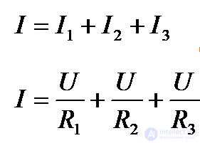
Then 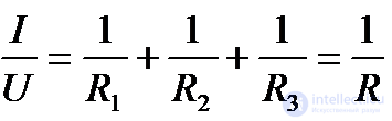 (1.30)
Thus, the reciprocal of the total (equivalent) resistance R of parallel-connected loads is equal to the sum of the reciprocals of the resistances of these loads.
The quantity that is the reciprocal of resistance determines the conductance of a load g. Then the total (equivalent) conductance of the circuit for parallel-connected loads is determined by the sum of the conductances of the loads
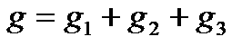 (1.31)
If n identical loads with resistance R/ each are connected in parallel, then the equivalent resistance of these loads is 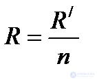 . If two loads with resistances R1 and R2 are connected in parallel, then their total (equivalent) resistance in accordance with (1.30) is equal to
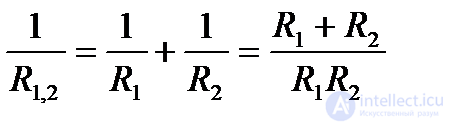
Hence 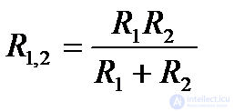 (1.32)
If three loads with resistances R1, R2, R3 are connected in parallel, then their total resistance (see (1.30))

Hence 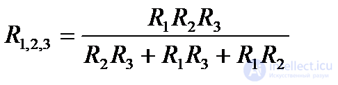 (1.33)
A change in the resistance of any one of the parallel-connected loads does not affect the operating mode (voltage) of the other loads, including the one being changed. This is why parallel connection has found wide practical application.
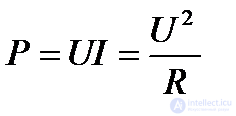
When loads are connected in parallel, less power is dissipated in the larger resistance:
Potential diagram
When studying and calculating certain electric circuits, it is necessary to determine the potentials of individual points of the circuit and construct a potential diagram. For this, expression (3.4) can be used (Fig. 3.1a).

On section AB, point B has a positive potential  , point A has a negative potential
  , therefore
  , since the source operates in generator mode, i.e.
 .
.
On section BC, point B has a positive potential , point C has a negative potential , therefore  , the source with EMF E2 operates in consumer mode, i.e.
 .
.
Thus, the potential of point D can be written as
 ,
,
if the circuit is traversed in the direction of the current, or
 ,
,
if the circuit is traversed against the direction of the current.
From this we can draw the following conclusion (rule): if a circuit or a section of a circuit is traversed in the direction of the current, then the potential at each point is determined by the potential of the previous point plus the EMF of a source operating in generator mode, minus the EMF of a source operating in consumer mode, and minus the voltage drop across the section between the points of the circuit.
When the loop is traversed against the direction of the current, the signs of the EMF and the voltage drop are reversed.
This rule is especially convenient to apply in cases where the circuit contains sections with several sources.
A potential diagram is a plot of the potentials of the circuit points against the values of the resistances of the sections between these points.
To construct a potential diagram, one of the points of the electric circuit is conventionally grounded (its potential is taken as zero), and the potentials of the remaining points equal the voltage between them and the grounded point.
A potential diagram is a broken (polygonal) line (Fig. 3.3).
Example 3.2
For the circuit shown in Fig. 3.2, given:
E1 = 8 V; E2 = 24 V; E3 = 9.5 V; R1 = 0.5 Ω; R2 = 1 Ω; R3 = 1.5 Ω; R01 = 0.15 Ω; R02 = 0.1 Ω; R03 = 0 Ω.
1. Determine the magnitude and direction of the current in the circuit.
2. Determine the potential of points B, C, D, E, G, taking the potential of point A as zero, 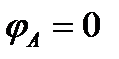 .
.
3. Construct the potential diagram.
4. Compose and verify the power balance for the circuit.
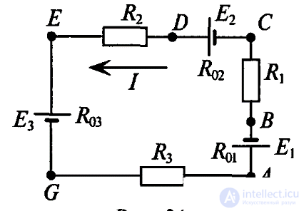
Fig. 3.2.
Solution
1. Let us choose the direction of loop traversal to be clockwise; then the magnitude of the current

The «minus» sign obtained as a result of the calculation indicates that the current is directed opposite to the chosen direction of traversal, as shown in Fig. 3.2. In the further calculations the «minus» sign is not taken into account. Thus, the EMF source E2 operates in generator mode, while E1 and E3 operate as consumers.
2. To determine the potentials of the indicated points, we traverse the loop in the direction of the current. This gives






3. To construct the potential diagram, the potentials of the points are plotted to scale along the ordinate axis, and the resistances of the sections along the abscissa axis. The potential diagram is shown in Fig. 3.3.
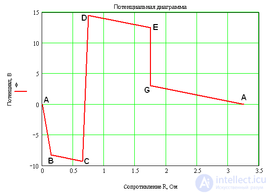
Fig. 3.3
4. The power balance in an electric circuit with several sources is satisfied provided that the sum of the powers of the sources operating in generator mode equals the sum of the powers of the sources operating in consumer mode, plus the power losses in all the resistances of the circuit, including the internal resistances of the sources:


48 W = 48 W.
Example 2.
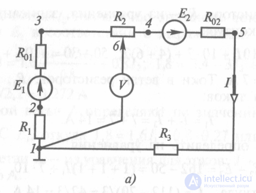
Calculate and plot the potential diagram for a DC electrical circuit (Fig. 1.19, a), given: the EMFs of the power sources E1 = 16 V; E2 = 14 V, internal resistance R01 = 3 Ω; R02 = 2 Ω, resistor resistances R1 = 20 Ω; R2 = 15 Ω; R3 = 10 Ω. Determine the position of the potentiometer wiper at which voltmeter V reads zero, and draw up the power balance for the circuit. How will the choice of a different zero-potential point affect the shape of the potential diagram?
b)
Fig. 1.19.
Solution. The current in the circuit is determined from the equation, derived from Kirchhoff's second law, reduced to the form:

The potential diagram is plotted in a rectangular coordinate system. Here, the resistances of all sections of the circuit are plotted along the abscissa axis to an appropriate scale, and the potentials of the corresponding points are plotted along the ordinate axis. When constructing the potential diagram, one of the circuit's points is conventionally grounded, i.e. it is assumed that its potential φ = 0. On the diagram, this point is placed at the origin of coordinates.
In accordance with the problem statement, the potentials of points 1 - 5 of the electrical circuit are determined, and the potential φ1 of point 1 of the circuit is taken as equal to zero.
The potential φ2 of point 2 is found from the expression written according to Kirchhoff's second law for section 1 - 2 of the circuit:
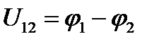
from which  .
.
Coordinates of point 2: R = 20 Ω; φ2 = -12 V.
According to Kirchhoff's second law, the following equation holds for section 1 - 3 of the circuit:
 ,
,
from which the potential of point 3 of the circuit is:  .
.
Coordinates of point 3 of the circuit: R = 20 + 3 = 23 Ω; φ3 = 2,2 V. The potential of point 4 of the circuit is determined similarly:
 ,
,
from which  .
.
Coordinates of point 4 of the circuit: R = 23 + 15 = 38 Ω; φ4 = - 6,8V.
The potential φ5 of point 5 of the circuit is found from the equation written according to Kirchhoff's second law for section 4 - 5 of the circuit:
 ,
,
from which  .
.
Coordinates of point 5 of the circuit: R = 38 + 2 = 40 Ω; φ5 = 6 V. The potential φ1 of point 1 of the circuit is found from the equation written according to Kirchhoff's second law for section 4 - 5 of the circuit:  ;
;  . Coordinates of point 1 of the circuit: R = 40 + 10 = 50 Ω; φ1 = 0.
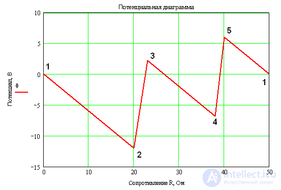
For the electrical circuit under consideration, the potential diagram based on the calculation results is shown in Fig. 1.19, b.
From this diagram it follows that the position of the potentiometer wiper at point 6 of the circuit corresponds to a voltmeter reading of zero, since the potentials of points 1 and 6 of the circuit are equal.
When a different zero-potential point of the electrical circuit is chosen, the potential differences across the corresponding sections of the circuit do not change, since they are determined by the magnitude of the current and the magnitude of the resistance. If the potential of point 3 of the circuit φ3 = 0 is taken, then the abscissa axis shifts to point 3 of the potential diagram (dashed line), i.e. the potentials of all points of the circuit decrease by the value of the potential φ, equal to segment 0K = 2,3 V.
The power balance corresponds to the following equation:
 ;
;
16 ∙ 0,6 + 14 ∙ 0,6 = 0,62(20 + 3 + 15 + 2 + 10).
18 W = 18 W.
Let us consider a parallel connection of resistances, in which all branches of the electrical circuit (consumers) are under the same voltage (Fig. 2.22).
For the schematic diagram of a parallel connection of elements, let us write Kirchhoff's first law in complex form:

The current vectors (phasors) in the parallel branches:

where 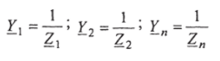 - are the total complex admittances of the 1st, 2nd, ... nth branches;
 are the total complex impedances of the 1st, 2nd, ... nth branches.
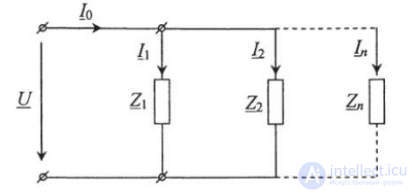
Fig. 2.22. Schematic diagram of a parallel connection of loads
Total current in the circuit:
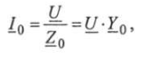
where  is the total complex admittance of the parallel connection;
 is the total complex impedance of the parallel connection.
Obviously,
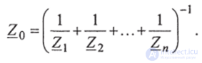
Let us determine the admittance for branch 1 

Multiplying the numerator and denominator of equation (2.38) by 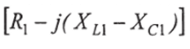 we get:
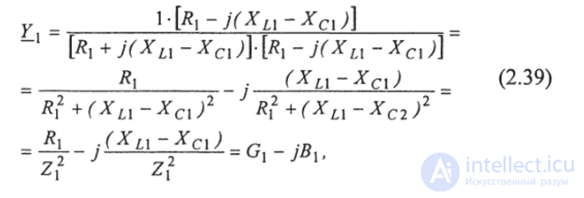
where  - the square of the magnitude of the total impedance of branch 1;
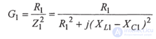 - the active conductance of branch 1;
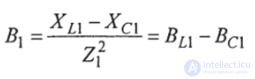 - the reactive susceptance of branch 1.
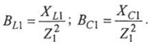
Taking into account relations (2.39), the total admittance for branch 1 can be written as follows:
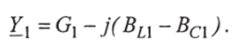
Then the magnitude of the total admittance of branch 1

On the complex plane (Fig. 2.23), the terms of the circuit's complex admittance are shown as vectors for two cases: BL1 > Bc1 (Fig. 2.23a) and BL1 < Bc1 (Fig. 2.23b). In the first case, the circuit's complex admittance is inductive in nature; in the second, it is capacitive.
If the circuit's complex admittance is inductive in nature, then the total current (in the unbranched part of the circuit) lags the voltage in phase, since  .
.
If the circuit's complex admittance is capacitive in nature, then the total current leads the voltage in phase, since  .
.
Note that, as before, positive values of the angle  are measured counterclockwise from the vector of the complex current value
  or admittance
The admittance triangle for branch 1 is shown in Fig. 2.23c:
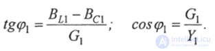
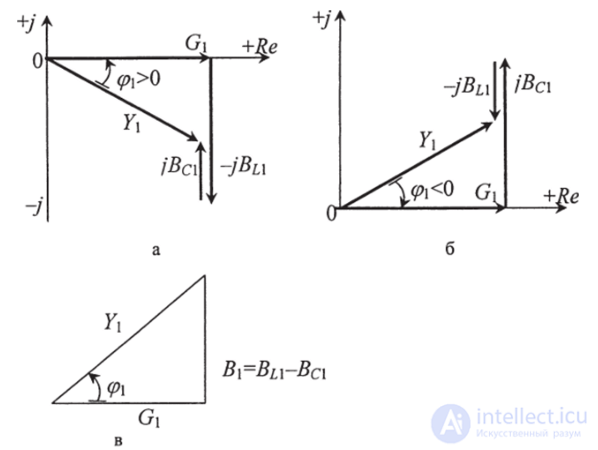
Fig. 2.23. Admittances for branch 1 on the complex plane:
BL1 > Bc1 (Fig. 2.23a)
BL1 < Bc1 (Fig. 2.23b)
admittance triangle (c)
Similarly, the admittances for all other branches are found and admittance triangles are constructed. Consequently, the admittance for the entire circuit
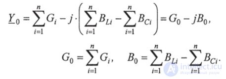
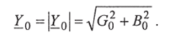
The magnitude of the total admittance of the entire circuit:
Example 2.6. According to the circuit (Fig. 2.24), given:

Determine: 
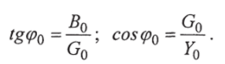
From the admittance triangle for the parallel circuit (Fig. 2.25) let us determine the angle 
Solution.
1. We find the complex admittance of the circuit:
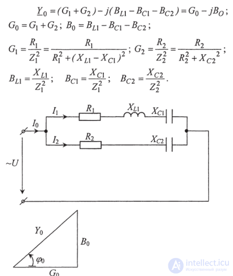
Fig. 2.24. Parallel circuit diagram
Fig. 2.25. Admittance triangle of the parallel circuit (Fig. 2.24)
2. We find the magnitude of the complex admittance of the circuit:

3. We find the complex current drawn by the circuit from the energy source: 
where 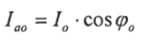 - the active component of the current
  ;
;
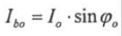 - the reactive component of the current
  ;
;
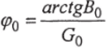 - the angle between U0 and /0.
4. The current complexes and /2 are equal:
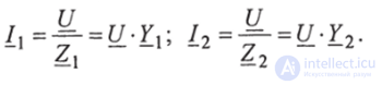
5. By Kirchhoff's first law, the current /0 is equal to:
The vector diagram for 
a circuit with a parallel connection of elements, shown in Fig. 2.26, is conveniently constructed relative to the voltage vector, since with this connection the voltage vector is common to all
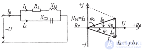
Fig. 2.26. Diagram of a parallel connection of elements
Fig. 2.27. Vector diagram for a parallel connection of branch elements. It is directed along the positive real axis (Fig. 2.27).
Let us write the equations for current and voltage for the circuit in Fig. 2.26 in complex form:
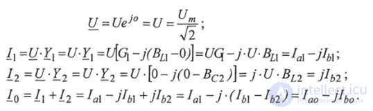
On the vector diagram in Fig. 2.27, the currents according to the equations in branches 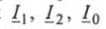 are represented in algebraic form as the sum of the active components of the currents,
  which are found as the projections of the corresponding current vectors onto the real-number axis Re, and the reactive components of the currents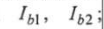
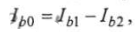 , which are found as the projections of the corresponding currents onto the imaginary-number axis (j).
The active and reactive components of the currents are found using the formulas:


Comments