
Lecture
An important fundamental question in the theory of discretization is the question of the volume of the discrete description of signals, that is, the number  of basis functions used for the representation:
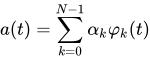 .
.
To find the optimal basis, one must define the class of signals for which it is being sought, and also specify the required reconstruction accuracy for that class. Under a statistical approach to describing signals, the optimal — dimensional basis for representing individual signal realizations is usually taken to be the basis for which the error norm, averaged over the ensemble of realizations, is minimal. In this case the necessary and sufficient conditions for the minimum error norm of a signal representation as a sum of basis functions are given by the Karhunen-Loève theorem.
The minimum value of the error norm for representing signals on an interval of length  is achieved when the basis used consists of the eigenfunctions of the operator whose kernel is the correlation function of the signals
  :
:
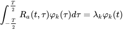 ,
,
corresponding to the largest eigenvalues. In this case the error norm equals:
 .
.
Such an expansion is a Karhunen-Loève expansion .
In the theory of random processes, the Karhunen-Loève theorem (named after Kari Karhunen and Michel Loève) — is a representation of a random process as an infinite linear combination of orthogonal functions, analogous to a Fourier series representation — the sequential representation of functions on a bounded interval. Unlike a Fourier series, where the coefficients are real numbers and the representation basis consists of sinusoidal functions (that is, of sine and cosine functions of different frequencies), the coefficients in the Karhunen-Loève theorem — are random variables, and the representation basis depends on the process. The orthogonal basis functions used in this representation are determined by the covariance function of the process. If we regard a stochastic process as a random function F, that is, a process in which the function on the interval [a, b] takes the value F, then this theorem can be viewed as a random orthonormal expansion of F.
A centered random process {Xt}t ∈ [a, b] (where centered means that the expectations E(Xt) exist and equal zero for all values of the parameter t in [a, b]), satisfying a technical continuity condition, admits an expansion of the following form:
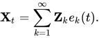
where Zk — are mutually uncorrelated random variables and the functions ek — are continuous real-valued functions on [a, b], orthogonal in L² [a, b]. In the case of a non-centered process, an analogous expansion holds, obtained by expanding the mean function in the basis ek.
If the process  is Gaussian, then the random variables Zk — are also Gaussian and independent. This result generalizes the Karhunen-Loève transform. An important example of a centered random process on the interval [0,1] is the Wiener process, and the Karhunen-Loève theorem can be used to obtain its canonical orthogonal representation. In this case the expansion consists of sinusoidal functions.
The expansions given above are also known as Karhunen-Loève expansions or decomposition (the empirical version, that is, with coefficients derived from the original numerical data), as principal component analysis, proper orthogonal decomposition, or the Hotelling transform.
Let us state the result in terms of complex-valued stochastic processes. The results can be applied to real-valued processes without modification, recalling that the complex conjugate of a real number coincides with the number itself.
For random elements X and Y, the inner product is defined by the formula

where * denotes the complex conjugation operation.
The inner product is well-defined if both  and
and  have finite second moments, or, equivalently, if they are both square-integrable. Note that the inner product is related to the covariance and correlation. In particular, for random variables with zero mean, the covariance and the inner product coincide. The autocovariance function




If the process {Xt}t is centered, then

for all t. Thus the autocovariance KXX equals the autocorrelation RXX:

Note that if {Xt}t is centered and t1, ≤ t2, …, ≤ tN are points on the interval [a, b], then it follows that

Theorem. Consider a centered random process  , indexed by
  on the interval
  with covariance function
  . Suppose that the covariance function
  is jointly continuous in the variables
  . Then — is a positive-definite kernel, and by Mercer's theorem the integral operator on
  (close to Lebesgue measure on ) has an orthonormal basis of eigenvectors. Let
  be the eigenvectors of corresponding to nonzero eigenvalues, and
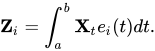
Then  — are centered orthogonal random variables, and
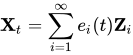
the series converges in mean square, and also uniformly in . Moreover

where  is the eigenvalue corresponding to the eigenvector
  .
.
In the statement of the theorem, the integral in the definition of can be understood as the mean limit of Cauchy sums of random variables
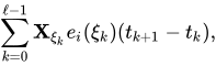
where

Since the mean-square limit of jointly Gaussian random variables is Gaussian, and jointly Gaussian (centered) random variables are independent if and only if they are orthogonal, we may also conclude:
Theorem. The random variables have a Gaussian distribution and are independent if the original process {Xt}t is also Gaussian.
In the Gaussian case, since the random variables are independent, we can be certain that:
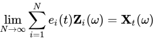
almost surely.
Note that, generalizing Mercer's theorem, we can replace the interval with other compact spaces  , and the Lebesgue measure on — with a Borel measure supported on .
The Wiener process in the theory of random processes — is a mathematical model of Brownian motion, or a continuous-time random walk. Here we define it as a centered Gaussian process B(t) with covariance function

It is easy to see that the eigenvectors of the covariance are
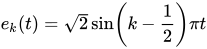
and the corresponding eigenvalues are
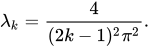
This allows us to obtain the following representation of the Wiener process:
Theorem. There exists a sequence {Wi}i of independent Gaussian random variables with zero mean and unit variance such that
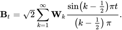
The convergence is uniform in t in the L² norm, so that
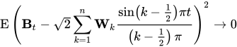
uniformly in t.
It has been suggested that the SETI project should use Karhunen-Loève transforms to detect signals with a very broad spectrum. Similarly, adaptive optics systems sometimes use Karhunen-Loève functions to reconstruct information about the wavefront phase. (Dai 1996, JOSA A).

Comments