Filtration. Markov Times, Stopping Time. Examples

Markov time (in the theory of stochastic processes) — is a random variable that does not depend on the future of the stochastic process under consideration.

Discrete case

Let a sequence of random variables be given. Then the random variable is called a Markov time (moment) if, for any , the event depends only on the random variables .

Example

Let — be a sequence of independent normal random variables. Let , and

— the first time the process reaches the level . Then — is a Markov time, since if and only if there exists such that . Thus the event depends only on the behavior of the process up to the time .

Let now

— the last time the process reaches the level . Then is not a Markov time, since the event presupposes knowledge of the future behavior of the process.

General case

• Let a probability space be given with a filtration , where . Then the random variable taking values in is called a Markov time with respect to this filtration if .

• If a process is given, and — are its natural σ-algebras, then — is said to be a Markov time with respect to the process .

• A Markov time is called a stopping time if it is finite almost surely, that is

.

Properties

If and — are Markov times, then

• — is a Markov time;
• — is a Markov time;
• — is a Markov time.

Remark: a stopping time may not have a finite expectation.

Example

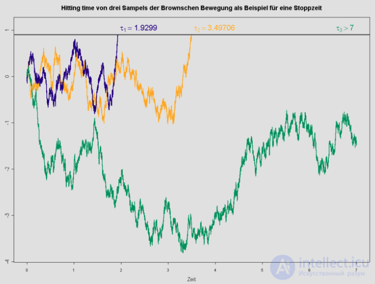
Let — be a standard Wiener process. Let . Define

.

Then — is a Markov time whose distribution is given by the probability density

.

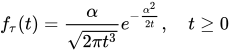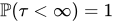
In particular, — is a stopping time. However,

.

Markov times.

3.1. Definition. Let - the random variable is called a Markov time, if 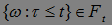for .

A finite Markov time is called stopping time (i.e. ).

Example. Let be right-continuous with values in then the first time of reaching the level : , is a Markov time.

Theorem 10. 1) Let be a Markov time, then
2) Let be a Markov time, then .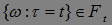

Proof. 1) Since is a Markov time, 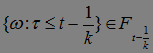. Hence for we obtain .

2) Since , the assertion follows from part 1). The proof is complete.

Theorem 11. If and are Markov times, then: 1) is a Markov time, 2) is a Markov time.

Prove this on your own.

3.2. A natural question arises: under what conditions is the random variable a Markov time?

Theorem 12. The random variable is a Markov time if for .

Proof. Since is a random variable, 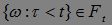. Let us prove that . From the definition of a random variable it follows that 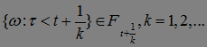Intersecting all these sets, we have 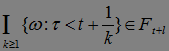, for . Therefore, by the conditions of the theorem, we have .The proof is complete.

Theorem 13. If there are two Markov times, then and are Markov times.

Prove this on your own.

3.3. Definition. Let — be Markov times (M. t.), where P - a. s.. The sets

are called, respectively, right-open, left-open, right- and left-open, closed stochastic intervals, and are denoted, respectively, by

By we denote the set and call it the graph of the Markov time .

Problem. Prove that .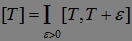

3.4. Definition. A random set A is called thin, if it has the form , where is a sequence of stopping times. If, in addition, the sequence is such that 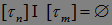as , then such a sequence is called exhausting for the set A.

Theorem 14. The thin set A and all its sections 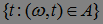are at most countable, moreover, there exists an exhausting sequence of stopping times.

3.5. Definition. A random process is called stopped if .

Definition. Let a sequence of Markov times be such that , where P -a. s. for and let
P - a. s.. We call such a sequence localizing (). If, on the other hand, , then the sequence is called localizing.

Definition. A random process is called a local martingale, if there exists a localizing sequence of Markov times such that for P - a. s. .

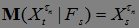A local submartingale and supermartingale are defined analogously.

Theorem 15. Let be a local martingale with respect to the measure P. Then is a supermartingale (with respect to the measure P).

Proof. Since P — a.s. for , where is a localizing sequence, then by Fatou's lemma .
The proof is complete.

3.6. Let us now turn to the classification of Markov times.

3.6.1. Definition. A Markov time is called predictable, if there exists a sequence of Markov times such that: a) P - a. s., b) P - a. s., and the sequence is called announcing the Markov time .

Example. Let be a stopping time, and . It is clear that is a stopping time, moreover is a predictable stopping time, since is announced by the sequence , where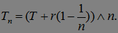

Definition. A Markov time is called accessible, if there exists a predictable sequence of Markov times such that P - a. s., i. e.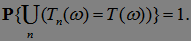

3.6.2. Definition. A Markov time is called inaccessible (totally or completely inaccessible) or optional, if for every predictable stopping time 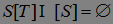P - a. s. .

Problem. Prove that if a Markov time is simultaneously accessible and totally inaccessible, then P - a. s..

Theorem 16. A Markov time is optional if and only if there exists a sequence of stopping times such that: a) P - a. s. for , b) P - a. s..

Prove this on your own.

The following statement is obvious.

Theorem 17. Let — be an optional Markov time. Then for any predictable sequence of Markov times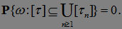

Problem. Prove that the moment of time at which the first jump of the Poisson process occurs is an optional Markov time.

Theorem 18. Let 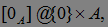where , and stochastic intervals of the form , where are optional Markov times, generate the -algebra .

Proof. First note that is a predictable stopping time equal to zero on and to infinity on . Hence . It is clear that . Note that is a predictable M. t., hence 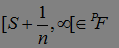, and therefore .

Consider the interval , where is a predictable M. t. We need to show that this interval belongs to the -algebra generated by the intervals considered above. Indeed, since , and for the sequence , announcing on the set , we have 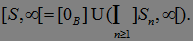This proves the assertion of the theorem.

Examples and applications

To illustrate some examples of random times where the rules stop, and some where they do not, consider a gambler playing roulette with a typical casino advantage, starting with $100 and betting $1 on red in each game:

• Exactly five games corresponds to the stopping time τ = 5 and are a stopping rule.
• Playing until he runs out of money or plays 500 games, is a stopping rule.
• Playing until he reaches his maximum score so far is not a stopping rule and does not define a stopping time, since it requires information about the future as well as the present and past.
• Playing until he doubles his money (borrowing if necessary) , is not a stopping rule, since there is a positive probability that he will never double his money.
• Playing until he doubles his money or runs out of money, is a stopping rule, even though there is potentially no limit on the number of games he plays, since the probability that he stops after a finite time is 1.

To illustrate a more general definition of stopping time, consider Brownian motion, which is a random process., where each is a random variable defined on the probability space . We define a filtration on this probability space by letting- the σ -algebra generated by all sets of the form where and is a Borel set. Intuitively, the event E is inif and only if we can determine whether E, is true or false simply by observing the Brownian motion from time 0 to time t .

• Every constant (trivially) is a stopping time; this corresponds to the stopping rule "stop at time".
• Let then be a stopping time for Brownian motion, corresponding to the stopping rule: «stop as soon as the Brownian motion exceeds the value a ».
• Another stopping time is given by . This corresponds to the stopping rule: «stop as soon as the Brownian motion becomes positive over a continuous stretch of length 1 unit of time».
• In general, if τ ₁ and τ ₂ are stopping times on then their minimum , their maximum , and their sum τ ₁ + τ ₂ are also stopping times. (This is not true for differences and products, because they may require «looking into the future» to determine when to stop.)

A hitting time such as in the second example above can be an important example of a stopping time. Although it is relatively easy to show that essentially all stopping times are hitting times ^, it can be much harder to show that a given hitting time is a stopping time. The latter kinds of results are known as the Debut theorem .

Types of stopping times

Stopping times with a fixed time index I = [0, ∞) are often divided into one of several types depending on whether it is possible to predict when they are about to occur.

A stopping time τ is predictable , if it is equal to the limit of an increasing sequence of stopping times т _п , satisfying т _п < т , whenever τ > 0. The sequence τ _п is said to announce τ and predictable stopping times are sometimes called announceable . Examples of predictable stopping times are hitting times of continuous and adapted processes. If τ is the first time that a continuous real-valued process X equals some value a, then it is announced by the sequence τ _n , where τ _n is the first time that X is within a distance of 1 / n from a .

Accessible stopping time is a time that can be covered by a sequence of predictable times. That is, a stopping time τ is accessible if P ( τ = τ _n for some n ) = 1, where τ _n are predictable times.

A stopping time τ is totally inaccessible , if it can never be announced by an increasing sequence of stopping times. Equivalently, P ( τ = σ <∞) = 0 for every predictable time σ . Examples of totally inaccessible stopping times include the jump times of Poisson processes .

Every stopping time τ can be uniquely decomposed into an accessible and a totally inaccessible time. That is, there exists a unique accessible stopping time σ and a totally inaccessible time υ such that τ = σ, if σ <∞, τ = υ, if υ <∞, and τ = ∞, if σ = υ = ∞. Note that in the statement of this decomposition result, stopping times need not necessarily be almost surely finite and may equal ∞.

Stopping rules in clinical trials

Clinical trials in medicine often carry out interim analyses to determine whether the trial has already reached its endpoints. However, interim analysis creates a risk of false-positive results, and therefore stopping boundaries are used to determine the number and timing of interim analyses (also known as alpha spending, to denote the rate of false positives). In each of the R interim tests, the trial is stopped if the probability falls below a threshold p, which depends on the method used.

Problems for independent solution

1. Let a filtration — be Markov times with respect to F.

Prove that

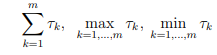
are also Markov times with respect to F.

2. Given a filtration and Markov times τ and σ with respect to it. For τ define the sigma-algebra

. Prove that if

See also

• Optimal stopping
• Odds algorithm
• Secretary problem
• Hitting time
• Stopped process
• Disorder problem
• Debut theorem
• Sequential analysis