
Lecture
In statistical radio engineering and physics, when studying deterministic signals and random processes, their spectral representation in the form of the spectral density, which is based on the Fourier transform, is widely used.
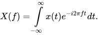
If the process  has finite energy and is square integrable (and this is a nonstationary process), then for a single realization of the process one can define the Fourier transform as a random complex function of frequency:
 |
(1) |
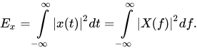
However, it turns out to be almost useless for describing the ensemble. A way out of this situation is to discard some of the spectrum parameters, namely the phase spectrum, and to construct a function characterizing the distribution of the process's energy over the frequency axis. Then, according to Parseval's theorem, the energy
 |
(2) |
The function 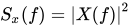 thus characterizes the distribution of the realization's energy over the frequency axis and is called the spectral density of the realization. By averaging this function over all realizations one can obtain the spectral density of the process.
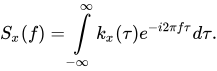
Let us now turn to a wide-sense stationary centered random process {\displaystyle x(t)}, whose realizations, with probability 1, have infinite energy and, consequently, have no Fourier transform. The power spectral density of such a process can be found, on the basis of the Wiener-Khinchin theorem, as the Fourier transform of the correlation function:
 |
(3) |
If the direct transform exists, then the inverse Fourier transform also exists, which from the known  determines
  :
:
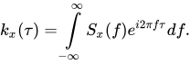 |
(4) |
If we set in formulas (3) and (4), respectively,  and
and  , we have
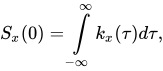 |
(5) |
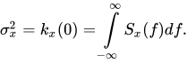 |
(6) |
Formula (6), together with (2), shows that the variance determines the total energy of the stationary random process, which is equal to the area under the spectral density curve. The dimensional quantity  can be interpreted as the fraction of energy concentrated in a small frequency interval from {\displaystyle f-df/2}
 to
to  . If {\displaystyle x(t)} is understood as a random (fluctuating) current or voltage, then the quantity {\displaystyle S_{x}(f)} will have the dimension of energy [V2/Hz] = [V2s]. For this reason is sometimes called the energy spectrum. In the literature one often encounters another interpretation:
  – is regarded as the average power dissipated by the current or voltage across a 1-Ohm resistance. In this case the quantity is called the power spectrum of the random process.
 . . |
(7) |
 . . |
(8) |
and the energy spectrum of a wide-sense stationary random process possess all the properties characteristic of a pair of mutual Fourier transforms. In particular, the «wider» the spectrum the «narrower» the correlation function , and vice versa. This result is expressed quantitatively in the form of an uncertainty principle or relation.
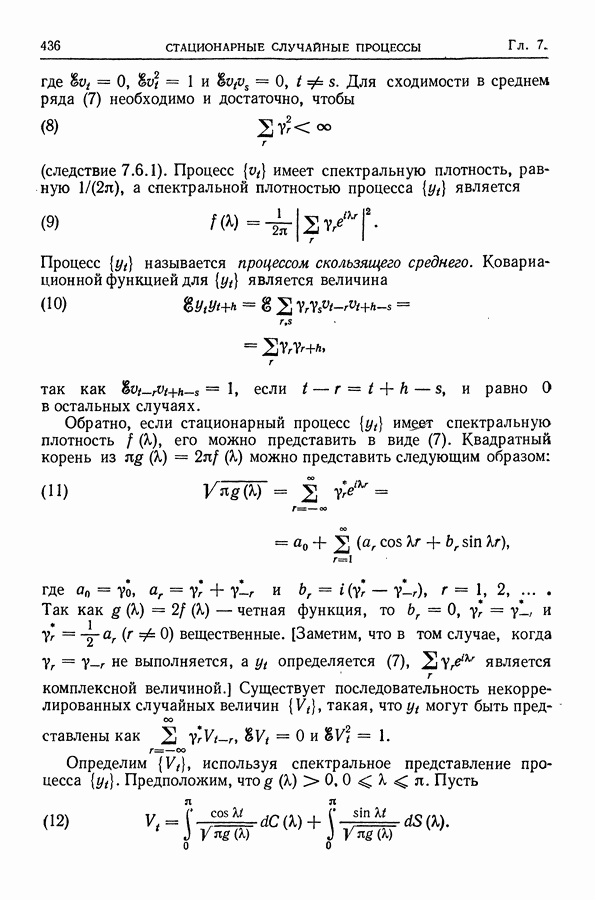
Suppose that  is a moving-average process of uncorrelated random variables
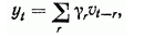
where  For convergence in the mean of series (7) it is necessary and sufficient that

(corollary 7.6.1). The process  has spectral density equal to
  and the spectral density of the process
  is
is
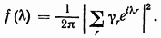
The process  is called a moving-average process. The covariance function for
  is the quantity
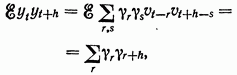
since  if
if  and equal to 0 otherwise.
Conversely, if a stationary process  has spectral density
  it can be represented in the form (7). The square root of
  can be represented as follows:
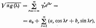
where  Since
Since  is an even function,
  are real. [Note that in the case when
  does not hold,
  defined by (7), is a complex quantity.] There exists a sequence of uncorrelated random variables
  such that
  can be represented as
Let us define  using the spectral representation of the process
  Suppose
  Let
Let 

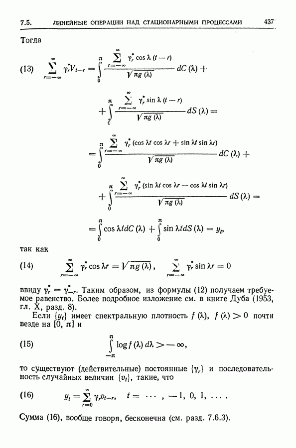
Then
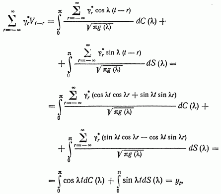
since

because of  Thus, from formula (12) we obtain the required equality. For a more detailed exposition, see Doob's book (1953, Ch. X, Sect. 8).
If  has spectral density
  almost everywhere on
  and
and
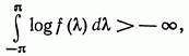
then there exist (real) constants  and a sequence of random variables
  such that

The sum (16) is, in general, infinite (see Sect. 7.6.3).
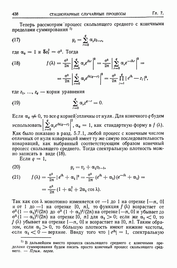
Now consider a moving-average process with finite limits of summation
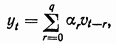
where  Then
Then
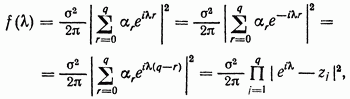
where  are the roots of the equation
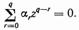
If  then all
  roots are nonzero. For finite
  we shall use
  as the standard form in
  As was shown in Sect. 5.7.1, any process with a finite number of nonzero covariances has the same sequence of covariances as a suitably chosen finite moving-average process. Then the spectral density can be written in the form (18). If
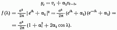
Since  varies monotonically from —1 to 1 on the interval
  and from 1 to —1 on the interval
  the function
  increases from
  to
to  on the interval
  and decreases to
  on the interval
  for
for  whereas if
  then
then  decreases on the interval
  and increases on
  Thus, if
  the lower frequencies have the greater density, while if
  the upper frequencies do. Since
  the spectral
density can be written as follows:
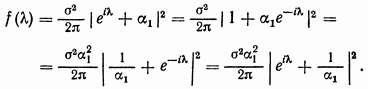
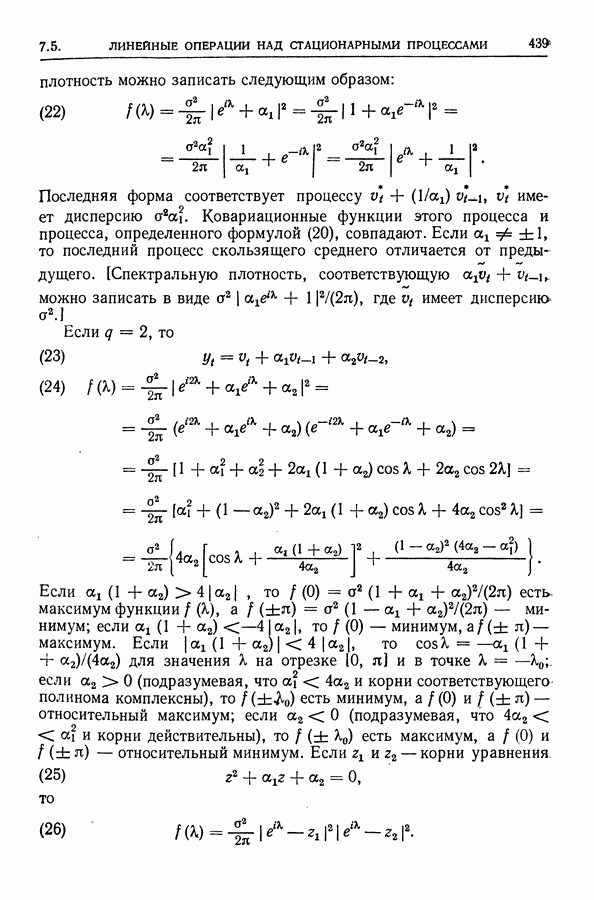
The latter form corresponds to a process  has variance
  The covariance functions of this process and of the process defined by formula (20) coincide. If
  , then the latter moving-average process differs from the former one. [The spectral density corresponding to
  can be written in the form
  where
where  has variance
  .]
.]
If
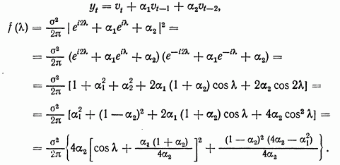
If  then
then  is a maximum of the function
  a minimum; if
  then
then  is a minimum,
  a maximum. If
  then
then  for values of X on the interval
  and at the point
  if
if  (implying that
  and the roots of the corresponding polynomial are complex), then
  is a minimum, and
  a relative maximum; if
  (implying that
  and the roots are real), then
  is a maximum, and
  a relative minimum. If
  are the roots of the equation

then

Since 1, the factor  can be replaced by
  where
where  is the conjugate of
  can be replaced by
  Thus, for the function
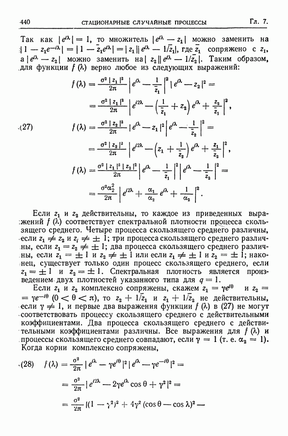
  any of the following expressions holds:
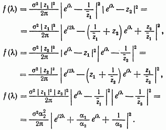
If  are real, then each of the expressions given for
  corresponds to the spectral density of a moving-average process. The four moving-average processes are distinct if
  three moving-average processes are distinct if
  two moving-average processes are distinct if
  or if
or if  finally, there is only one moving-average process if
  The spectral density is the product of two densities of the indicated type for
If  are complex conjugates, say
  then
then  are not real if
  and the first two expressions of the function
  in (27) cannot
  correspond to a moving-average process with real coefficients. Two moving-average processes with real coefficients are distinct. All expressions for
  and the moving-average processes coincide if
  (i.e.
(i.e.  When the roots are complex conjugates,
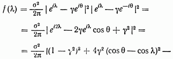

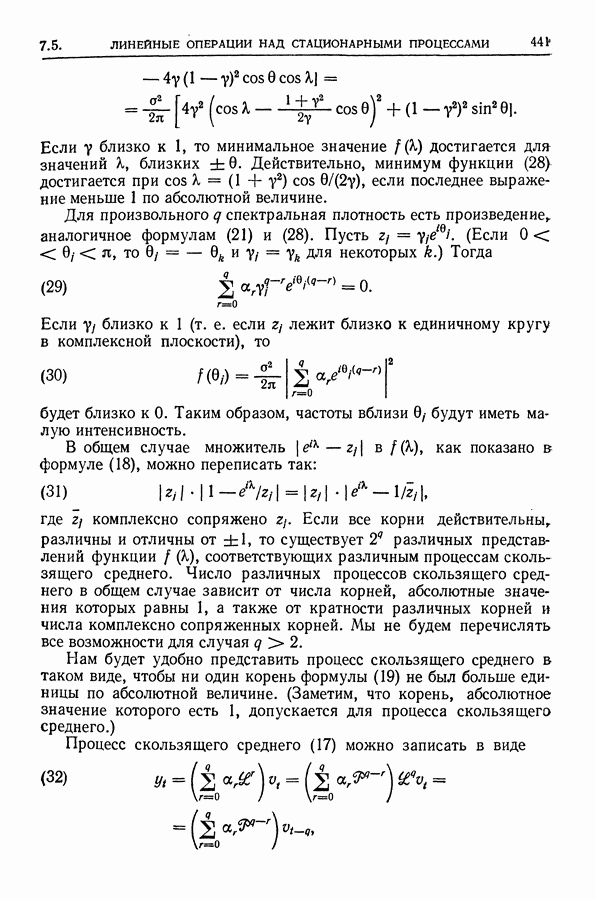
If y is close to 1, then the minimum value of  is attained for values of X close to ±0. Indeed, the minimum of function (28) is attained at
  if the latter expression is less than 1 in absolute value.
For arbitrary  the spectral density is a product analogous to formulas (21) and (28). Let
  (If
(If  then
then  For some
  Then
Then
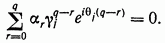
If  is close to 1 (i.e. if
  lies close to the unit circle in the complex plane), then
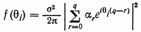
will be close to 0. Thus, frequencies near  will have low intensity.
In the general case, the factor  as shown in formula (18), can be rewritten as follows:

where  is the complex conjugate of
  If all the roots are real, distinct, and different from ±1, then there exist
  distinct representations of the function
  corresponding to different moving-average processes. The number of distinct moving-average processes in the general case depends on the number of roots whose absolute values equal 1, as well as on the multiplicity of the various roots and the number of complex conjugate roots. We shall not enumerate all the possibilities for the case
It will be convenient for us to represent the moving-average process in such a form that no root of formula (19) is greater than unity in absolute value. (Note that a root whose absolute value is 1 is permitted for a moving-average process.)
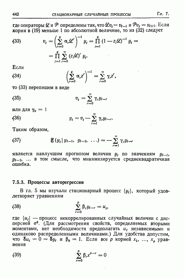
The moving-average process (17) can be written in the form
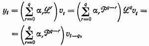
where the operators and  are defined so that
  If the roots in (19) are less than 1 in absolute value, then from (32) it follows that
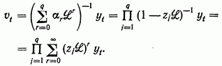
If
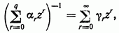
then (33) can be rewritten as
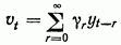
or
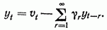
Thus,

is the best forecast of the quantities  in terms of the values
  in the sense that the mean-square error is minimized.

Comments