
Lecture
Gaussian processes. Construction of a real Gaussian process with given mean function and covariance function.
In probability theory and statistics, a Gaussian process — is a stochastic process (a collection of random variables indexed by some parameter, most often time or coordinates), such that any finite set of these random variables has a multivariate normal distribution, that is, any finite linear combination of them is normally distributed. The distribution of a Gaussian process – is the joint distribution of all its random variables and, as a consequence, is a distribution over functions with a continuous domain.
If a Gaussian process is regarded as a way of solving machine learning problems, then lazy learning is used together with a similarity measure between points (kernel function) to obtain a prediction of the value at an unseen point from the training set. The notion of a prediction, besides the point estimate itself, includes information about uncertainty — a one-dimensional Gaussian distribution.
To compute predictions for certain kernel functions, the method of matrix algebra, kriging, is used.
The Gaussian process is named in honor of Carl Friedrich Gauss, since it is based on the concept of the Gaussian distribution (normal distribution). A Gaussian process can be regarded as an infinite-dimensional generalization of multivariate normal distributions. These processes are used in statistical modeling; in particular, properties of normality are used. For example, if a random process is modeled as Gaussian, then the distributions of various derived quantities, such as the mean value of the process over a given interval of time and the error of its estimate obtained from a sample of values, can be derived explicitly.
A continuous-time random process is Gaussian if and only if, for any finite set of indices  from the index set

- is a multivariate Gaussian random variable. Equivalently, every linear combination 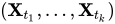 has a one-dimensional normal (Gaussian) distribution. Using the characteristic functions of random variables, the Gaussian property can be formulated as follows:
  is Gaussian if and only if, for any finite set of indices , there exist real values
  ,
,  where
where  such that for all
  the equality holds

Where  - is the imaginary unit.
The numbers and - are the covariances and mean values of the variables in the processes, respectively.
The key distinguishing feature of Gaussian processes is that they can be fully specified by second-order statistics. Consequently, the covariance function fully determines the behavior of the process, given that the expectation of the Gaussian process is zero. It is important to note that the non-negative definiteness of the function makes possible its spectral decomposition via the Karhunen — Loève expansion. Through the covariance function one can define the stationarity, isotropy, smoothness, and periodicity of the process.
Stationarity expresses the behavior of the process with respect to the distance between any two points  and
and  . If the process is stationary, then it depends on the relative arrangement of its points, the distance between them,
  , otherwise it is non-stationary, that is, it depends on the actual positions of the points and . An example is provided by a particular case of the Ornstein — Uhlenbeck process, the Brownian motion process: it is stationary.
If the process depends only on  , the Euclidean distance (not the direction) between and , then the process is considered isotropic. A stationary and isotropic process is called homogeneous; in practice, the properties of stationarity and isotropy reflect the differences (or, rather, the lack thereof) in the behavior of the process with respect to the position of the observer.
The essence of Gaussian processes lies in obtaining prior probability distributions whose smoothness depends on the chosen covariance function. If we expect that for input points that "lie close" and the corresponding output points  and
and  also "lie close," then an assumption of continuity of the function is present. If we want to allow a significant deviation, then a coarser covariance function must be chosen. As examples of extreme behavior, one can cite the Ornstein — Uhlenbeck covariance function and the squared exponential function, where the former is nowhere differentiable, while the latter is infinitely differentiable.
Periodicity refers to inducing periodic patterns in the behavior of the process. Formally, this is achieved by mapping the input value onto a two-dimensional vector

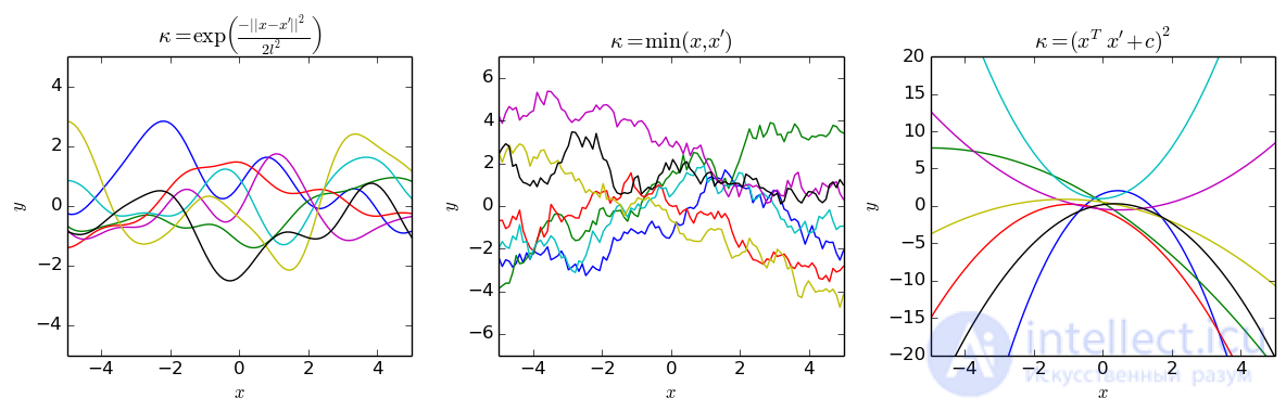
The effect of choosing different kernels on the distribution function of a Gaussian process. Left to right: squared exponential kernel, Brownian, quadratic
There exist a number of common covariance functions:
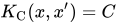


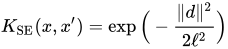
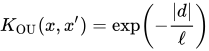

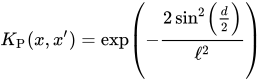

Here  . The parameter
  is a characteristic of the length scale of the process (practically, «how close» two points and must be in order to significantly influence one another),
  - is the Kronecker symbol and
  - is the standard deviation of the noise fluctuations. Furthermore,
  is the modified Bessel function
  and
and  - is the gamma function evaluated at . It is important to note that a complex covariance function can be defined as a linear combination of other, simpler covariance functions in order to combine different information about the available datasets.
Obviously, the results obtained depend on the values of the hyperparameters  (for example, and ), which determine the behavior of the model.
The Wiener process (the so-called Brownian motion) is the integral of a white-noise Gaussian process. It is not stationary, however it has stationary increments.
The Ornstein — Uhlenbeck process — is a stationary Gaussian process.
The Brownian bridge (similar to the Ornstein — Uhlenbeck process) is an example of a Gaussian process whose increments are not independent.
Fractional Brownian motion is a Gaussian process whose covariance function is a generalization of the covariance function of the Wiener process.
A Gaussian process can be used as a prior probability distribution over functions in Bayesian inference. For any set of N points in the desired function domain, take a multivariate Gaussian distribution whose covariance matrix parameter is the Gram determinant of the N points taken with some desired kernel, and a sample from that distribution.
Inference of continuous values based on a Gaussian process determined by prior covariances is known as kriging (Gaussian process regression). Gaussian processes are therefore useful as a powerful nonlinear multivariate interpolation tool. Gaussian process regression can be further extended to solve both supervised and unsupervised (self-learning) learning problems.
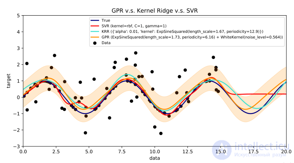
An example of Gaussian process regression compared with other regression models.
When discussing the fundamental problem of Gaussian process regression (kriging), it is assumed that for a Gaussian process  , observed at coordinates , the vector of values
  is merely one sample from a multivariate Gaussian distribution whose dimensionality equals the number of observed coordinates
  . Hence, under the assumption of a zero-mean distribution,
  , where
  - is the covariance matrix between all possible pairs of
  for a given set of hyperparameters . Thus, the log marginal likelihood is equal to:

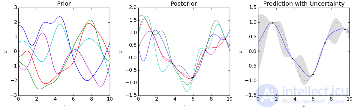
Gaussian process regression (prediction) with a squared exponential kernel
and maximizing this marginal likelihood with respect to gives a complete characterization of the Gaussian process . It can be noted that the first term depends on the inability of the model to fit the observed values, while the second term is directly proportional to the complexity of the model. Having specified and made a prediction of the unobserved values  at coordinates
  , it remains to plot samples from the predictive distribution
  , where the posterior mean estimate
  is defined as

and the posterior variance estimate B is defined as

where  - is the covariance between the new coordinate estimate and all other observed coordinates for a given hyperparameter vector , and are defined as before, and
  is the variance at point , dictated by the vector . It is important to note that the posterior mean estimate (a "point estimate") is a linear combination of the observations ; similarly, the variance does not actually depend on the observations . A well-known bottleneck in Gaussian process prediction is that the computational complexity of prediction is cubic in the number of points , that is, the computation may be infeasible for large datasets. To circumvent this problem, work is being done on sparse Gaussian processes, which are usually based on the idea of constructing a representative set for the given process . [10]

Comments