
Lecture
Martingales, submartingales, supermartingales. Examples. Doob decomposition.
§ 3 Martingales, supermartingales, submartingales.
3.1. Let ( ,
, ,
, ,P) – be a stochastic basis, the sequence {
 is adapted to the flow , and takes values in
  .
.
Definition. The sequence ( ,
, )t>1 is called a martingale if:
1) 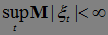 , 2)
, 2) 
If 1) holds and 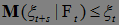 P -a. s., then the sequence (,)t>0 is called a supermartingale.
If 1) holds and 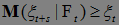 P - a. s., then the sequence (,)t>0 is called a submartingale.
Example. Let  , where
  are jointly independent random variables. Let
  ,
, 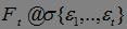 . It is clear that
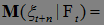


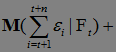 =
=
=+ +
+  +
+ .
.
It follows that:
a) (,)t>1- is a martingale, if  for any t;
b) (,)t>1- is a supermartingale, if  for any t;
c) (,)t>1- is a submartingale, if  for any t;
Proposition 5. If (,)t>0– is a Markov random sequence with transition probability P(s, ,t,B), then
P(s,  t,B) – is a martingale for
  , with respect to the flow
  of algebras
 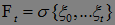 and the measure P.
Proof. From the Chapman – Kolmogorov relation we have
P-a. s. for  :
:
M(P(u,  ,t,B)|
 )=M(P(u, ,t,B)|
  ) =
) =  .
.
3.2. Theorem 6 (Doob). Let (,)t>0 – be a nonnegative supermartingale, then with probability 1 there exists  .
.
Remarks. 1) Let us show that the assumption of nonnegativity of the supermartingale (,)t>0 can be dropped. It is obvious that M M
M , i.e. on average the sequence
  - decreases. Let
  Form a new sequence
  . It is clear that
  .Then
.Then 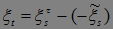 , hence any supermartingale can be represented as the difference of two nonnegative supermartingales.
2) If  - supermartingale, then
  - is a submartingale. Hence the assertion of Theorem 6 also holds for submartingales.
3.2.1 The proof of Doob's theorem relies on two auxiliary lemmas.
Let  be a numerical sequence, a<b, [a,b] – an interval. Denote by
  the number of upcrossings of the interval [a,b] by the sequence
  .
.
Lemma 7 (On the number of upcrossings of the interval [a,b]).
The following inequality holds:
 ,
,
where 

Proof. Denote
 ,
,  ,
,
 ,
,  ,
,

 ,
, 
It is obvious that 
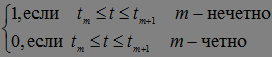
It follows that
(b-a)  =
=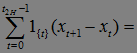
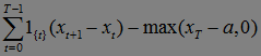 .
.
The proof is complete.
Lemma 8. (On the mean number of upcrossings). Let (,)t>0– be a nonnegative supermartingale, then M
 .
.
Proof. By Lemma 7 we have the inequality:
 .
.
Since (,)t>0 - is a supermartingale, M( ) ≤ 0. It follows that the inequality

 . The proof is complete.
3.2.2. Proof of Theorem 6. Suppose that the sequence  has no finite limit. Denote by B the set
  has no finite limit}. Our assumption holds if:
1)  P - a. s.,
2) 
 P - a. s.
Denote: A
 }, C=
}, C=
 }. It is obvious that
  , hence
  . So to prove the theorem it suffices to prove that P(A) =0 and P(C)=0.
Let us show that P(A)=0. By Chebyshev's inequality and Fatou's lemma we have P(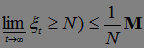


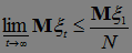 . Letting now
  , we obtain P(A)=0.
Now let us prove that P(C)=0. Note that
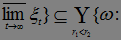
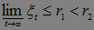
 , where
  and
and  are rational numbers}=
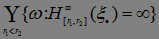 =
=
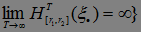 .
.
Consider the probability P( N); by Chebyshev's inequality and Lemma 8 we have:
P( N)
N) .
.
Letting now  , we obtain the inequality
  P(
P( N)
N) . It follows that P(
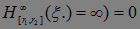 , i.e.P(C)=0. The proof is complete.
3.3. Definition. A martingale  is called uniformly integrable, if
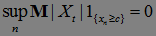 .
.
Theorem 9. Let be a uniformly integrable martingale, then P -a.s. there exists a random variable 
 such that:
a) =  P - a. s.,
b)  M|-
M|- P - a. s.
The proof of this theorem follows from Theorem 6.
Doob martingale in the theory of stochastic processes — is a random process constructed in a sufficiently general way that always turns out to be a martingale.
Let an arbitrary sequence of random variables  be given. Let the random variable
  be such that its expectation is finite:
  . Define the sequence
 .
.
Then the random process  is a martingale and is called the Doob martingale.
In the theory of discrete-time stochastic processes, which is part of the mathematical theory of probability, the Doob decomposition theorem gives a unique decomposition of every adapted and integrable stochastic process into the sum of a martingale and a predictable process (or «drift»), starting from zero. The theorem was proved by Joseph L. Doob and is named in his honor.
The analogous theorem in the continuous-time case is the Doob – Meyer decomposition theorem.
Let (Ω, F , ℙ) be a probability space, I = {0, 1, 2 ,. . . , N } with N ∈ ℕ or I = ℕ 0 a finite or infinite index set, ( F n ) n ∈ I a filtration of F , and X = ( X n ) n ∈ I an adapted random process with E [| X n |] <∞ for all n ∈ I . Then there exists a martingale M = ( M n ) n ∈ I and an integrable predictable process A = ( A n ) n ∈ I , starting from A 0 = 0 , such that X n = M n + n for any n ∈ I . Here predictable means that n is F n -1 -measurable for any n ∈ I \ {0 }. This decomposition is almost surely unique.
The theorem holds verbatim also for stochastic processes X, taking values in the d -dimensional Euclidean space ℝ d or the complex vector space ℂ d . This follows from the one-dimensional case by considering the components individually.
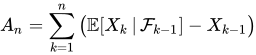
Using conditional expectations, define the processes A and M for each n ∈ I explicitly as
 1
1
and 2
2
where the sums for n = 0 are empty and are defined to be zero. Here A adds up the expected increments of X , while M adds up the surprises, i.e. the part of each X k, that is not known one time step earlier. From these definitions, A n + 1 (if n + 1 ∈ I ) and M n are P n -measurable, because the process X is adapted, E [| A n |] <∞ and E [| M n |] <∞ , since the process X is integrable, and the decomposition X n = M n + n holds for any n ∈ I . Martingale property
 since
since
also follows from the definition ( 2 ) given above, for any n ∈ I \ {0 }.
To prove uniqueness, let X = M ' + A ' be another decomposition. Then the process Y : = M - M ' = A ' - A is a martingale, from which it follows that
 since,
and is also predictable, implying that
 since
since
for any n ∈ I \ {0 }. Since Y 0 = A ' 0 - A 0 = 0 by convention on the starting point of predictable processes, this iteratively implies that Y n = 0 almost surely for all n ∈ I , hence the decomposition is almost surely unique.
A real-valued stochastic process X is a submartingale if and only if it has a Doob decomposition into a martingale M and an integrable predictable process A, which is almost surely nondecreasing. It is a supermartingale if and only if A is almost surely nonincreasing.
If X is a submartingale, then
 since
since
for all k ∈ I \ {0 }, which is equivalent to the statement that every term in the definition ( 1 ) of A is almost surely positive, hence A is almost surely nondecreasing. The equivalence for supermartingales is proved analogously.
Let X = ( X n ) n ∈ℕ 0 be a sequence of independent integrable real-valued random variables. They are adapted to the filtration generated by the sequence, i. E. F n = σ ( X 0 , ..., X n ) for all n ∈ ℕ 0 . According to ( 1 ) and ( 2 ) the Doob decomposition is given by

and

If the random variables of the original sequence X have zero mean, this simplifies to
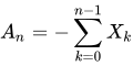 and
and 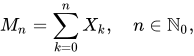
hence both processes are (possibly time-inhomogeneous) random walks . If the sequence X = ( X n ) n ∈ℕ 0 consists of symmetric random variables taking the values +1 and −1 , then X is bounded, but the martingale M and the predictable process A are unbounded simple random walks (and not uniformly integrable ), and Doob's optional stopping theorem may not apply to the martingale M, if the stopping time does not have finite expectation.
In financial mathematics, the Doob decomposition theorem can be used to determine the largest optimal exercise time of an American option . Let X = ( X 0 , X 1 , ..., X N ) denote the nonnegative discounted payoffs of an American option in an N- period financial market model adapted to the filtration ( F 0 , F 1 ,. ..., F N ) , and let ℚ denote an equivalent martingale measure . Let U = ( U 0 , U 1 ,..., U N ) denote the Snell envelope of X with respect to ℚ . The Snell envelope is the smallest ℚ- supermartingale dominating X, and in a complete financial market it represents the minimum amount of capital needed to hedge the American option until maturity. Let U = M + A denote the Doob decomposition with respect to with of the Snell envelope U into the martingale M = ( M 0 , M 1 , ..., M N ) and the decreasing predictable process A = ( A 0 , A 1 , ..., A N ) with A 0 = 0 . Then the largest stopping time for the optimal exercise of the American option is given by

Since A is predictable, the event { τ max = n } = { A n = 0, A n +1 <0 } lies in F n for any n ∈ {0, 1,. . . , N - 1 }, so τ max is indeed a stopping time. It is the last moment before the discounted value of the American option is expected to drop; up to the moment τ max the discounted value process U is a martingale with respect to ℚ .
The Doob decomposition theorem can be generalized from probability spaces to σ-finite measure spaces .

Comments