
Lecture
. The concept of stochastic differential equations and strong solutions.
A stochastic differential equation ( SDE ) is a differential equation in which one or more of the terms is a stochastic process, resulting in a solution that is also a stochastic process. SDEs are used to model various phenomena, such as unstable stock prices or physical systems subject to thermal fluctuations. Typically, SDEs contain a variable which represents random white noise, calculated as the derivative of Brownian motion or a Wiener process. However, other types of random behavior are possible, for example, jump processes. Random differential equations are conjugate to stochastic differential equations.
Stochastic differential equations originated in the theory of Brownian motion, in the work of Albert Einstein and Smoluchowski. These early examples were linear stochastic differential equations, also called «Langevin» equations after the French physicist Langevin, describing the motion of a harmonic oscillator subject to a random force. The mathematical theory of stochastic differential equations was developed in the 1940s through the pioneering work of the Japanese mathematician Kiyosi Itô, who introduced the notion of the stochastic integral and initiated the study of nonlinear stochastic differential equations. A different approach was later proposed by the Russian physicist Stratonovich, leading to a calculus analogous to ordinary calculus.
It is customary to distinguish two types of solutions of stochastic differential equations: strong and weak solutions.
The conditions imposed in the work of Skorokhod, Stroock and Varadhan, and Krylov were considerably weaker than Itô's conditions. Some ambiguity arose as to how the solution should be understood. A.N. Shiryaev and M.P. Ershov introduced the notions of strong and weak solution. The corresponding definitions are given in the book by R.Sh. Liptser and A.N. Shiryaev [14]. According to this terminology, the solution constructed by Itô is a strong solution, while the solutions constructed in later works (and under weaker assumptions) are weak. The relationship between strong and weak solutions is examined in the paper by A.K. Zvonkin and N.V. Krylov
in order for the existence theorem for solutions of stochastic differential equations to cover solutions analogous to sliding regimes for ordinary differential equations, for example motion along a surface on which the drift coefficient f is discontinuous and the diffusion coefficient g is zero, it is necessary to pass, just as
and for ordinary differential equations, to the corresponding stochastic differential inclusions. Since obtaining sliding regimes specifically is often the goal of control, because they depend weakly on external disturbances, proving existence theorems for such solutions is an important task. Considerable attention is devoted in the book to questions of the existence of solutions of various types of stochastic differential equations.
Weak solutions are used in studying those properties of equations that are connected with the measure on the space of trajectories, such as the stability of processes, the probabilistic representation of solutions, etc. But if it is necessary to consider a specific property of trajectories, for example in the control theory of diffusion processes or in filtering theory, then strong solutions are considered. In proving existence theorems for strong solutions, an important role is played by the Yamada-Watanabe principle: from the existence of weak solutions and pathwise uniqueness, strong existence follows. Note that the principle applies in various situations: for stochastic differential equations, for stochastic differential equations with reflection at the boundary, and for stochastic differential inclusions. The problem of existence and uniqueness of solutions of stochastic differential equations can be described as follows. There are equations that have no weak solutions. There are equations that have weak solutions on some probability space with a suitable Brownian motion, while on other probability spaces with other Brownian motions solutions may fail to exist. If pathwise uniqueness holds and the equation has the property of weak existence, then on any probability space with any Brownian motion there exists a unique solution, and it is strong.
The most common form of an SDE in the literature is an ordinary differential equation with a right-hand side perturbed by a term depending on a white-noise variable. In most cases, an SDE is understood as the continuous-time limit of the corresponding stochastic difference equations. This understanding of an SDE is ambiguous and must be supplemented by a rigorous mathematical definition of the corresponding integral. Such a mathematical definition was first proposed by Kiyosi Ito in the 1940s, leading to what is known today as Ito calculus. Later the Russian physicist Stratonovich proposed a different construction, which led to the so-called Stratonovich integral. The Ito integral and the Stratonovich integral are related to one another, but are different objects, and the choice between them depends on the application under consideration. Ito calculus is based on the concept of non-anticipativeness, or causality, which is natural in applications where time is a variable. In Stratonovich calculus, on the other hand, there are rules that resemble ordinary calculus, and there are intrinsic geometric properties that make it more natural for solving geometric problems, such as random motion on manifolds.
An alternative view of an SDE is as a stochastic flow of diffeomorphisms. This understanding is unambiguous and corresponds to the Stratonovich version of the continuous-time limit of stochastic difference equations. Associated with the SDE is the Smoluchowski equation or the Fokker – Planck equation, an equation describing the time evolution of probability distribution functions. The generalization of Fokker – Planck evolution to the time evolution of differential forms is provided by the concept of the stochastic evolution operator.
In physical science, the use of the term «Langevin SDE» is ambiguous. Although Langevin SDEs can take a more general form, the term usually refers to a narrow class of SDEs with gradient-flow vector fields. This class of SDEs is especially popular because it is the starting point of the Parisi – Sourlas stochastic quantization procedure, leading to a supersymmetric N = 2 model closely related to supersymmetric quantum mechanics. However, from a physical point of view this class of SDEs is not very interesting, because it never exhibits spontaneous breaking of topological supersymmetry, i.e. (overdamped) Langevin SDEs are never chaotic.
Brownian motion, or the Wiener process, turned out to be exceptionally difficult mathematically. The Wiener process is almost surely nowhere differentiable; it thus requires its own rules of calculation. There are two dominant versions of stochastic calculus, Ito stochastic calculus and Stratonovich stochastic calculus. Each has its own advantages and drawbacks, and beginners often do not understand which one is better suited to a given situation. Guidelines exist (for example, Øksendal, 2003), and for convenience an Ito SDE can easily be converted into an equivalent Stratonovich SDE and back. Nevertheless, one must be careful which calculus is used when an SDE is first written down.
Numerical methods for solving stochastic differential equations include the Euler-Maruyama method, the Milstein method, and the Runge-Kutta method (SDE).
In physics, SDEs have an extremely wide range of applications - from molecular dynamics to neurodynamics and the dynamics of astrophysical objects. In particular, SDEs describe all dynamical systems in which quantum effects are either unimportant or can be accounted for as perturbations. SDEs can be regarded as a generalization of dynamical systems theory to models with noise. This is an important generalization, since real systems cannot be completely isolated from their environment and for this reason always experience external stochastic influence.
There are standard methods for converting higher-order equations into several coupled first-order equations by introducing new unknowns. Thus, the most general class of SDE is:

where - is the position of the system in its phase space (or state space), assumed to be a differentiable manifold, - is the flow vector field representing the deterministic law of evolution, and - is a set of vector fields that define the coupling of the system to Gaussian white noise, . If this is a linear space and are constants, the system is said to be subject to additive noise; otherwise it is said to be subject to multiplicative noise. This term is somewhat misleading, since it has come to mean the general case, although it seems to imply the limited case in which . 


For a fixed noise configuration, the SDE has a unique solution that is differentiable with respect to the initial condition. The nontriviality of the stochastic case becomes apparent when one attempts to average various objects of interest over noise configurations. In this sense, the SDE is not an unambiguously defined object when the noise is multiplicative and when the SDE is understood as the continuous-time limit of a stochastic difference equation. In this case the SDE must be supplemented by so-called «SDE interpretations», such as the Ito or Stratonovich interpretations of the SDE. Nevertheless, when the SDE is regarded as a continuous-time stochastic flow of diffeomorphisms, it is an unambiguously defined mathematical object that corresponds to the Stratonovich approach to the continuous-time limit of the stochastic difference equation.
In physics, the main method of solution is to find the probability distribution function as a function of time using the equivalent Fokker – Planck equation (FPE). The Fokker – Planck equation is a deterministic partial differential equation. It tells how the probability distribution function evolves in time, much as the Schrodinger equation gives the time evolution of the quantum wave function or the diffusion equation gives the time evolution of chemical concentration. Alternatively, numerical solutions can be obtained by Monte Carlo simulation. Other methods include path integration, based on the analogy between statistical physics and quantum mechanics (for example, the Fokker-Planck equation can be transformed into a Schrodinger equation by rescaling several variables), or by writing ordinary differential equations for the statistical moments of the probability distribution function.
The notation used in probability theory (and in many applications of probability theory, for example in financial mathematics) differs slightly. This is also the notation used in publications on numerical methods for solving stochastic differential equations. This notation makes more explicit the exotic character of the random function of time in the physics formulation. In strict mathematical terms, it cannot be chosen as an ordinary function, but only as a generalized function. The mathematical formulation treats this complication with less ambiguity than the physics formulation. 
A typical equation has the form

where denotes the Wiener process (standard Brownian motion). This equation should be interpreted as an informal way of expressing the corresponding integral equation

The above equation characterizes the continuous-time behavior of the random process X t as the sum of an ordinary Lebesgue integral and an Ito integral. A heuristic (but very useful) interpretation of the stochastic differential equation is that over a small time interval of length δ the stochastic process X t changes its value by an amount that is normally distributed with expectation μ ( X t , t ) δ and variance σ ( X t , t ) 2 δ and does not depend on the behavior of the process in the past. This is because the increments of the Wiener process are independent and normally distributed. The function μ is called the drift coefficient, and σ - the diffusion coefficient. The random process X t is called a diffusion process and satisfies the Markov property .
A formal interpretation of the SDE is given in terms of what constitutes a solution of the SDE. There are two main definitions of a solution of an SDE: a strong solution and a weak solution. Both require the existence of a process X t, that solves a version of the integral equation of the SDE. The difference between them lies in the underlying probability space ( ). A weak solution consists of a probability space and a process satisfying the integral equation, whereas a strong solution is a process that satisfies the equation and is defined on a given probability space. 
An important example is the equation of geometric Brownian motion

which is the equation for the dynamics of a stock price in the Black – Scholes option pricing model in financial mathematics.
There are also more general stochastic differential equations in which the coefficients μ and σ depend not only on the current value of the process X t , but also on previous values of the process and, possibly, on current or previous values of other processes. In this case the solution process X is not Markovian and is called an Ito process rather than a diffusion process. When the coefficients depend only on the present and past values of X , the defining equation is called a stochastic delay differential equation.
As in the case of deterministic ordinary and partial differential equations, it is important to know whether a given SDE has a solution and whether it is unique. Below is a typical existence and uniqueness theorem for Ito SDEs taking values in n -dimensional Euclidean space R n and driven by m -dimensional Brownian motion B ; a proof can be found in Øksendal (2003, §5.2).
Let T > 0 and let


- be measurable functions for which there exist constants C and D , such that


for all t ∈ [0, T ] and all x and y ∈ R n , where
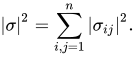
Let Z - be a random variable that is independent of the σ- algebra generated by B s , s ≥ 0, and with finite second moment:
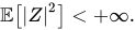
Then the stochastic differential equation / initial value problem


has a P-almost surely unique t -continuous solution ( t, ω ) ↦ X t ( ω ) such that X is adapted to the filtration F t Z , generated by Z and B s , s ≤ t and
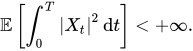


where


for a given differentiable function is equivalent to the Stratonovich SDE 

which has the general solution

where
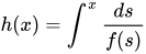

for a given differentiable function is equivalent to the Stratonovich SDE

which reduces to

where where is defined as before. Its general solution: 


In the supersymmetric theory of SDEs, stochastic dynamics is defined through a stochastic evolution operator acting on differential forms on the phase space of the model. In this exact formulation of stochastic dynamics, all SDEs possess a topological supersymmetry, which represents the preservation of the continuity of phase space by the continuous flow of time. The spontaneous breaking of this supersymmetry is the mathematical essence of the ubiquitous dynamical phenomenon known across disciplines as chaos, turbulence, self-organized criticality, etc., and Goldstone's theorem explains the associated long-range dynamical behavior, that is, the butterfly effect, 1/f and crackling noise, and the scale-free statistics of earthquakes, neuroavalanches, solar flares, etc. The theory also offers a resolution of the Ito–Stratonovich dilemma in favor of the Stratonovich approach.

Comments