
Lecture
Random walk — a mathematical object, known as a stochastic or random process, that describes a path consisting of a sequence of random steps in some mathematical space (for example, on the set of integers).
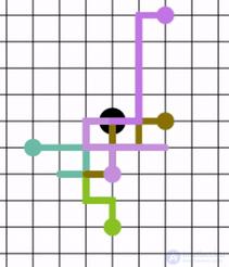
Five random walks of eight steps starting from a central point. Some paths appear shorter than 8 steps: in this case, the path retraces some of the steps in the opposite direction.
The simplest example of a random walk is a random walk on the integer number line ,  , which starts at point 0 and at each step shifts by +1 or −1 with equal probability. Other examples might include the trajectory of a molecule moving in a liquid or gas (Brownian motion), the path-finding of animals while foraging, fluctuations in stock prices on the financial market, or the financial state of a gambler: all of these cases can be approximated by random walk models, even though they may not be fully random in real life.
As the examples show, the random walk model is applied in engineering and many scientific fields, including ecology, psychology, computer science, physics, chemistry, biology, economics, and sociology. Random walk explains the observed behavior of many processes in these fields, and thus serves as a fundamental model for recorded stochastic activity. Thus, in mathematics, the value of π can be approximated using a random walk and agent-based modeling. The concept of random walk was first introduced by Karl Pearson in 1905.
Types of random walk can be of various kinds of interest. The term itself most often refers to a special category of Markov chains or a Markov process, while many time-dependent processes are referred to as random walks with a modifier indicating their special properties. Random walks (Markovian or not) can also occur in a variety of settings: those commonly studied include graphs, the integer or real number line, vector spaces, curved surfaces, higher-dimensional Riemannian manifolds, as well as finite, finitely generated groups, and Lie groups. The time parameter can also vary. In the simplest case, the walk takes place in discrete time and is a sequence of random variables (Xt) = (X1, X2, ...) indexed by natural numbers. However, there also exist random walks in which the steps occur at arbitrary moments in time, in which case the position X
t must be defined for all moments of time t ∈ [0,+∞). Special cases of random walk include the Lévy flight and diffusion models such as Brownian motion.
Random walk is a fundamental topic in discussions of Markov processes, and its mathematical study is very extensive.
A well-known random walk model is the walk on a regular lattice, where at each step the location moves to another point according to some probability distribution.
In a simple random walk, the location can move only to neighboring points of the lattice, forming a lattice path. In a simple symmetric random walk on a locally finite lattice, the probabilities of the point moving to each of its immediate neighbors are equal. The most studied example is the random walk on the d-dimensional integer lattice (sometimes called the hypercubic lattice)  .
.
If the state space is bounded to a finite number of dimensions, such a random walk model is called a simple bounded symmetric random walk, and the transition probabilities depend on the location of the point, because movement is restricted at boundary and corner points.
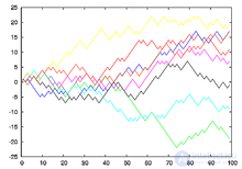
 of eight one-dimensional random walks.
The simplest example of a random walk is a random walk on the integer number line, , which starts at point 0 and at each step shifts by +1 or −1 with equal probability.
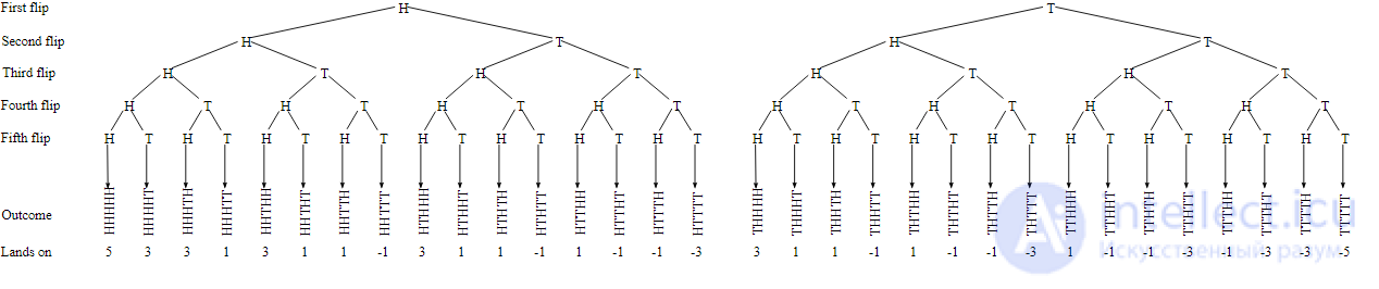
This walk can be illustrated as follows. A marker is placed at zero on the number line, and a «fair» coin is tossed. If it lands «heads», the marker moves one unit to the right, and if «tails» — one unit to the left. After five tosses, the marker can be at −5, −3, −1, 1, 3, 5. Out of five tosses, among which there are three «heads» and two «tails», occurring in any order, the marker will be at 1. There are 10 ways to end up at point 1 (by getting three «heads» and two «tails»), 10 ways to end up at point −1 (three «tails» and two «heads»), 5 ways to end up at point 3 (four «heads» and one «tails»), 5 ways to end up at point −3 (four «tails» and one «heads»), 1 way to end up at point 5 (five «heads»), and 1 way to end up at point −5 (five «tails»). The possible outcomes of five tosses are illustrated below.
To define this walk formally, take independent random variables  , where each variable equals either 1 or −1, with probability equal to 50 % for each value, the set
  and
and 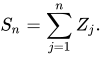 The series
  is called a simple random walk on . This series (the sum of a sequence of −1 and 1) represents the distance traveled, if each part of the walk has a length equal to one. The expected value
  of the series
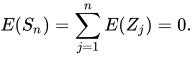
  is zero. That is, the mean value of all coin tosses tends to zero as the number of tosses increases. This follows from the property of finite additivity of expectation:
Reasoning similarly, using the independence of the random variables and the fact that  , we see:

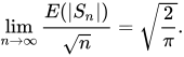
This makes clear that  , the expected distance after moving n steps, should be of order
  . In fact,
How many times will a random walk cross a boundary, if it is allowed to wander infinitely? The simplest random walk on will cross every point infinitely many times. This effect has many names: the level-crossing phenomenon, recurrence, or the gambler's ruin problem. The reason for the latter name is as follows: a gambler with a finite amount of money will sooner or later lose if he plays a fair game against a bank with an unlimited amount of money. The gambler's money represents a random walk, and at some point in time it will reach zero and the game will be over.
Let a and b — be positive integers, then the expected number of steps for a simple one-dimensional random walk starting at point 0 to first reach b or −a equals ab. The probability that this walk reaches b before it reaches −a equals  , which follows from the fact that a simple random walk is a martingale.
Some of the results mentioned above can be obtained from the properties of Pascal's triangle. The number of all distinct walks of n
steps, where each step is either +1 or −1, equals 2n. For a simple random walk, each of these steps is equally likely. For to equal the number k, it is necessary and sufficient that the number of +1 steps in the walk exceed the number of −1 steps by k. Hence, a +1 step must occur (n + k)/2 times among the n steps of the walk, hence, the number of walks satisfying the condition  , equals the number of ways to choose (n + k)/2 elements from an n-element set. This is denoted
 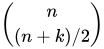 . For this expression to make sense, it is necessary that the sum n + k be an even number, which means that the numbers n and k must simultaneously be either even or odd. Consequently, the probability that equals
 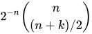 . Representing the entries of Pascal's triangle in terms of factorials and using Stirling's formula, one can obtain good estimates of these probabilities for large values of
  .
.
If, for brevity, we restrict the space to +, then the number of ways in which a random walk can stop at some number after five steps can be shown as {0,5,0,4,0,1}.
Let us demonstrate this correspondence to Pascal's triangle for small values of n. At step zero, the only possibility — is to remain at zero. However, already at the first move there is a possibility of ending up at either −1 or 1. At the second move, from 1 one can shift to point 2, or back to zero. From −1 one can shift to −2 or back to zero. Consequently, there is one case in which we end up at point −2, two cases in which we end up at zero, and one case — at point 2.
| k | −5 | −4 | −3 | −2 | −1 | 0 | 1 | 2 | 3 | 4 | 5 |
|---|---|---|---|---|---|---|---|---|---|---|---|
 |
1 | ||||||||||
 |
1 | 1 | |||||||||
 |
1 | 2 | 1 | ||||||||
 |
1 | 3 | 3 | 1 | |||||||
 |
1 | 4 | 6 | 4 | 1 | ||||||
 |
1 | 5 | 10 | 10 | 5 | 1 |
The central limit theorem and the law of the iterated logarithm describe important aspects of the behavior of a simple random walk on . In particular, as n increases, the probabilities (in proportion to the numbers in each row) tend toward a normal distribution.
A direct generalization can be considered to be random walks on crystal lattices (infinite abelian covering graphs of finite graphs). In fact, under such conditions it is even possible to establish the central limit theorem and the large deviation theorem.
The one-dimensional discrete random walk is a Markov chain with integer states, whose initial distribution is given by the probability function of the random variable  , and the transition probability matrix has the form
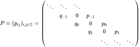 ,
,
that is



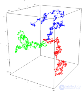
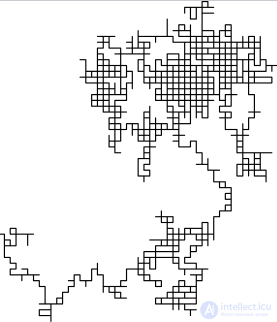
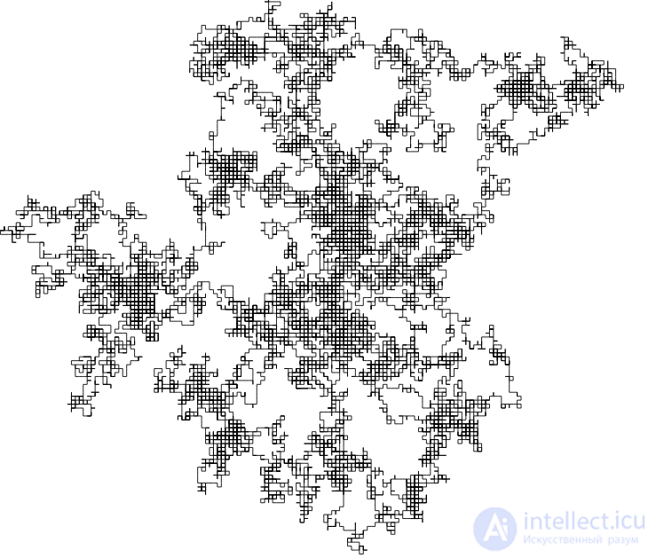
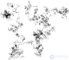
In higher dimensions, the set of points of a random walk has rather interesting geometric properties. In fact, we obtain a discrete fractal, that is, a set that exhibits stochastic self-similarity under increasing scale. At small scale, one can observe «raggedness» on the lattice along which the walk proceeds. Lawler's two books, listed in the references, are a good source of material on this topic. The trajectory of a random walk — is the collection of visited points, considered as a set up to the moment in time at which the walk reached the point. In one dimension, the trajectory is simply all the points between the minimum height and the maximum height that the walk has reached (both, on average, of order ).
To visualize the two-dimensional case, one can imagine a person randomly walking through a city. This city is effectively infinite and laid out on a square grid of sidewalks. At each intersection, the person randomly chooses one of four possible routes (including the one they came from). Formally, this is a random walk on the set of all points in the plane with integer coordinates.
Will this person ever return to the starting point of the walk? This case is the two-dimensional equivalent of the level-crossing problem discussed above. In 1921, György Pólya proved that the person will almost surely return in the case of a two-dimensional random walk, but for three dimensions or more, the probability of return decreases as the number of dimensions increases. In the three-dimensional case, the probability decreases to about 34 %. The mathematician Shizuo Kakutani is known for his quote about this result: «A drunk man will eventually find his way home, but a drunk bird may get lost forever».
Another variant of this question, also posed by Pólya, is this: if two people leave the same starting point, will they ever meet? One can reason that the difference between their locations (two independent random walks) is also a simple random walk, so they will almost surely meet in a two-dimensional walk, but for three dimensions or more, the probability of meeting, as in the previous case, decreases as the number of dimensions increases. Paul Erdős and Samuel James Taylor also showed in 1960 that for dimensions less than or equal to 4, two independent random walks, starting from any two given points, almost surely have infinitely many intersections, but for dimensions exceeding 5, they almost surely intersect only a finite number of times.
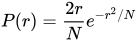
The asymptotic function for a two-dimensional random walk as the number of steps increases is given by the Rayleigh distribution. The probability distribution is a function of the radius from the origin, and for each step the step length is constant.
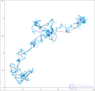
The Wiener process — is a stochastic process whose behavior resembles Brownian motion, the physical phenomenon of the diffusion of small particles in a liquid. (Sometimes the Wiener process is called Brownian motion, although, strictly speaking, the Wiener process is the model, while Brownian motion — is the phenomenon being modeled.)
The Wiener process — is the scaling limit of a one-dimensional random walk. This means that if one takes a random walk with very small steps, an approximation to the Wiener process can be obtained (and, with less precision, to Brownian motion). More precisely, if the step length equals ε, one must take a walk of length L/ε2 to approximate a Wiener path of length L. As the step length tends to zero (and the number of steps increases proportionally), the random walk converges to the Wiener process in the corresponding sense. Formally, if B is the space of all paths of length L with the maximum topology, and if M — is the space of measures over B with the normal topology, then convergence takes place in the space M. By analogy, the Wiener process in several dimensions is the scaling limit of a random walk in the same number of dimensions.
A random walk is a discrete fractal (a function with an integer number of dimensions; 1, 2, …), while the trajectory of a Wiener process — is a true fractal, and there is a definite connection between the two. For example, take a random walk and «step» until we cross a circle of radius r, multiplied by the step length. Then the average number of steps needed to complete the walk will equal r2. This fact — is a discrete version of the fact that the path of the Wiener process is a fractal of Hausdorff dimension 2.
In two-dimensional space, the average number of points that a random walk's path visits on the boundary of its trajectory equals r4/3. This corresponds to the fact that the boundary of the trajectory of the Wiener process is a fractal of dimension 4/3, which was conjectured by Mandelbrot using simulations, but was proven only in 2000 by Lawler, Schramm, and Werner.
The Wiener process has many symmetries, unlike a random walk. For example, the path of the Wiener process is invariant under rotation, whereas a random walk — is not, because its lattice is not invariant under rotation (a random walk is invariant under rotation by 90 degrees, whereas Wiener processes are invariant under rotation by, say, 17 degrees as well). This means that in many cases, problems posed in terms of a random walk are easier to solve as follows: transfer the problem to the Wiener process, solve it there, and then transfer it back. On the other hand, some problems are easier to solve using a random walk, thanks to its discrete nature.
The convergence of a random walk to a Wiener process is established by means of the central limit theorem and Donsker's theorem. For a particle at a known fixed position at t = 0, the central limit theorem tells us that after a large number of independent steps of the random walk, the position of the walker will be distributed according to a normal distribution of variance:

where t — is the time elapsed since the start of the random walk,  — is the size of a step in the walk, and
  — is the time elapsed between two consecutive steps.
This case corresponds to the Green's function of the diffusion equation, which describes the Wiener process, which allows us to suppose that after a sufficiently large number of steps, the random walk converges to the Wiener process.
In the three-dimensional case, the variance corresponding to the Green's function of the diffusion equation:

Equating this quantity with the variance associated with the position of the random walker, one can obtain the equivalent diffusion coefficient, considered for the asymptotic Wiener process to which the random walk converges after a sufficiently large number of steps:
 (makes sense only in the three-dimensional case).
Remark: the two variance expressions stated above correspond to the distribution associated with the vector  , which connects the two ends of the random walk in three dimensions. The variance associated with each component,
  ,
,  or
or  constitutes only one third of the total value (still 3D).
For 2D:

For 1D:

Consider a random walk  , where
  .
.
The central limit theorem states that 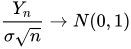 in distribution as
  .
.
However, for random walks this statement can be significantly strengthened.
Let us construct from  a random process
  , defining it as follows:
 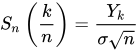 , and for the remaining
  we extend the process by linear continuation:

By the central limit theorem 
 in distribution as
This means convergence of the one-dimensional distributions of the process  to the one-dimensional distributions of the Wiener process. Donsker's theorem, also called the invariance principle, states that there is weak convergence of the processes,
Weak convergence of processes means convergence of functionals that are continuous with respect to the Wiener measure, that is, it allows the values of functionals of Brownian motion (for example, the maximum, the minimum, the last zero, the first hitting time of a level, and others) to be computed by a limiting transition from a simple random walk.
A random walk with a step length that varies according to a normal distribution is used to represent real-world time series data, such as financial markets. The Black — Scholes formula, for example, uses a Gaussian random walk as its basic assumption.
In this case the step size is the inverse cumulative normal distribution  where 0 ≤ z ≤ 1 and is a uniformly distributed random number, and μ and σ are the mean and standard deviation of the normal distribution, respectively.
If μ is nonzero, the random walk will depend on a linear trend (Eng. linear trend). If vs is the initial value of the random walk, then the expected value after n steps will equal vs + nμ.
For the special case where μ equals zero, after n steps, the probability distribution of the distance traveled is determined as N(0, nσ2), where N() is the notation for the normal distribution, n is the number of steps, and σ is taken from the inverse cumulative normal distribution mentioned above.
Proof: a Gaussian random walk can be represented as the sum of a sequence of independent and identically distributed random variables, Xi, from the inverse cumulative normal distribution, where the mean equals zero and σ is taken from the original inverse cumulative normal distribution:
Z =  ,
,
but we have the distribution for the sum of two independent normally distributed random variables, Z = X + Y, obtained thanks to
 (μX + μY, σ2X + σ2Y)
In our case, μX = μY = 0 and σ2X = σ2Y = σ2 give:
(0, 2σ2)
By induction, for n steps we have:
Z ~ (0, nσ2).
For steps distributed according to any distribution with zero mean and finite variance (not necessarily only the normal distribution), the root mean square of the distance traveled after n steps of the distance traveled is determined as:
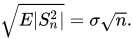
But for a Gaussian random walk this is just the standard deviation of the distribution of the distance traveled after n steps. Hence, if μ equals zero, and if the root mean square of the distance covered equals one standard deviation, there is a 68.27% probability that the root mean square of the distance covered after n steps will lie between ± σ. Also, there is a 50% probability that the distance traveled after n steps will lie between ± 0.6745σ.
In disordered systems, such as porous media and fractals,  may be proportional not to , but to
  . The exponent
  is called the anomalous diffusion exponent and can be greater or less than 2. Anomalous diffusion can also be expressed as σr2 ~ Dtα where α — is the anomaly parameter. Some diffusions in a random medium are even proportional to a power of the logarithm of time, for example Sinai's walk or Brox diffusion.
The number of sites distinct from one another visited by a single random walker  has been widely studied for square and cubic lattices and for fractals. This quantity is useful for analyzing trapping problems (Eng. trapping) and kinetic reactions. It is also related to the vibrational density of states, diffusion-reaction processes, and population distributions in ecology. The generalization of this problem to the number of distinct sites visited by
  random walkers, denoted as
  , has recently been studied for d-dimensional Euclidean lattices. The number of distinct sites visited by N walkers is not simply related to the number of distinct sites visited by each walker.
The estimate of the amount of information of a Gaussian random walk with respect to the squared error distance, that is, its quadratic distortion function, given parametrically:

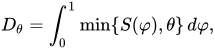
where  . Hence, it is impossible to binary-encode
  with fewer than
  bits and then decode it with an expected mean-square error less than
  . On the other hand, for any
  , there exists a sufficiently large
  and a binary code with no more than
  elements such that the expected mean-square error in reconstructing from this code is no more than
  .
.
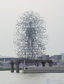
As already mentioned, the range of natural phenomena that various kinds of random walks have been used to describe is considerable. In particular, in physics, chemistry, materials science, biology, and various other sciences. Here are some applications of random walks:
In all of these cases the random walk is often replaced by Brownian motion:
Several kinds of random processes have been recognized as similar to pure random walks, but in which the simple structure may be more generalized. A pure structure can be characterized by steps determined by independent and identically distributed random variables.
A random walk of length k on a, possibly infinite, graph G rooted at 0 is a stochastic process with random variables  , such that
  , and
, and  is a vertex chosen uniformly at random among the neighbors of
  . Then the number
  — is the probability that a random walk of length k starts at v and ends at w. In particular, if G — is a graph rooted at 0,
  — is the probability that a random walk with step
  returns to 0.
By analogy with the previously described section (higher dimensions), suppose that our city no longer represents a perfect square grid. When our person reaches a certain intersection, they choose with equal probability among the different available roads. Thus, if there are seven exits at an intersection, the person will go to each one with probability one-seventh. In this way we obtain a random walk on a graph. Will our person get to their home? It turns out that, under fairly good conditions, the answer remains positive, but, depending on the graph, the answer to the next question ('Will two people meet?') «infinitely often» may no longer be an almost sure event.
An example where a person will almost surely get home is the case where the lengths of all blocks lie in the range from a to b (where a and b are two finite positive numbers). Important: we do not assume that the graph is planar, that is, tunnels and bridges may exist in the city. One way to prove this result — is by connecting it to electrical networks. Let us take a map of the city and place a resistor with a resistance of 1 ohm on each block. Now let us measure the «resistance between a point and infinity». In other words, let us choose some number R and take all points in the electrical network whose distance from our point is greater than R, and connect them together. We obtain a finite electrical network in which we can measure the resistance between our point and other points of the network. Let us send R to infinity. The resulting limit is called the resistance between a point and infinity.
It turns out that the following assumption is true (an elementary proof can be found in the book by Doyle and Snell):
Theorem: a graph is transient if and only if the resistance between a point and infinity is finite. Moreover, the choice of point does not matter if the graph is connected.
In other words, in a transient system, one only needs to overcome a finite resistance to reach infinity from any point. In a recurrent system, the resistance between any point and infinity is infinite.
A random walk on a graph is a special case of a Markov chain. Unlike a general Markov chain, a random walk on a graph has a property called temporal symmetry or reversibility. Roughly speaking, this property, also called the detailed balance principle, means that the probabilities of crossing a given path in one direction or the other have a very simple relationship between them (if the graph is regular, then they are equal). This property has important consequences.
Since the 1980s, much research has been carried out to relate graph properties to random walks. In addition to the electrical network described above, there are also connections to isoperimetric inequalities, functional inequalities such as the Sobolev and Poincare inequalities, and to the properties of solutions of Laplace's equation. A significant portion of such research has focused on Cayley graphs of finitely generated groups. In many cases these discrete results carry over to manifolds and Lie groups or are derived from them.
Speaking of random graphs, in particular the Erdos–Renyi model, analytical results have been obtained for some properties of random walkers. These include the distribution of the first and last hits (Eng. hitting time) of the walker, where the first hit is the first instance when the walker steps onto a previously visited site for the first time, and the last coincides with the case when the walker has nowhere left to go except to a previously visited site.
A good reference on random walks on graphs is the given online book. For studying groups, the books by Woess are suitable. If the transition kernel  is itself random (based on the environment
  ), then the random walk is called a «random walk in random environment». When the law of the random walk includes the randomness of , the law is called annealed (Eng. annealed); on the other hand, if is regarded as fixed, the law is called quenched (Eng. quenched).
We can choose every possible edge of the graph with the same probability, as the local maximum of uncertainty (entropy). We can also do this globally — in the maximal entropy random walk (Eng. maximal entropy random walk, MERW) it is required that all paths be equally probable or, in other words, for any two vertices, every path of a given length is equally probable. Such a walk has much stronger localizing properties.
There is a separate kind of random walk in which each step depends on the previous one in some complex way. They are more difficult to solve analytically than ordinary random walks; nevertheless, the behavior of any model of a random walker can be obtained using computers. For example:
A self-avoiding walk of length n on is a random path of length n steps, starting at the origin, that passes only through neighboring points in and never passes through the same point twice. In the two-dimensional case such a path is usually very short, while in higher dimension it grows without bound. This model is often used in polymer physics (since the 1960s).
Long-range correlated time series occur in many biological, climatological, and economic systems:
Random walks in which the direction of motion at one point in time correlates with the direction of motion at the next point in time. Used for modeling animal movements.

Comments