2.8 Characteristics of random variables associated with the renewal process

2.8 Characteristics of random variables associated with the renewal process

1. The epoch of the last renewal on a finite interval.

For a simple renewal process we study the distribution of the epoch of the last renewal on the interval [0,t). In this study the epoch t₀=0 is taken to be a renewal epoch in the situation where no renewals occurred on the interval [0,t).

Denote this epoch by ζ_t . Then obviously

P{ζ_t<0}=0, P{ζ_t=0}=1-F(t), P{ζ_tfor x>t . (2.35)

For 0<=t we obtain the equality

, (2.36)

if we take into account that dH(y) is the probability of a renewal occurring in the neighborhood of the point y, and 1-F(t-y) is the probability that there will be no renewals on (y,t), that is, that the last renewal before t occurred in the neighborhood of the point y. Equalities (2.35) and (2.36) solve the problem posed.

The distribution of the random variable ζ_t has a jump at zero (the jump size equals 1-F(t)) and is continuous at x=t , since

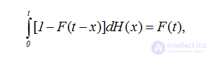
if we take into account equality (2.16).

From (2.36) we obtain

(2.37)

2. Backward recurrence time (undershoot time)

The backward recurrence time η_t (undershoot time) is defined as the time from the epoch of the last renewal occurring on the interval [0,t) to the epoch t. From the definitions it follows that a functional relation η_t+ζ_t=t holds between the random variables. Consequently, for

and from (2.35) and (2.36) we obtain

P{η_t <0}=P{ζ_t>t}=0, P{η_t =t}=P{ζ_t=0}=1-F(t),

P{η_t ζ_t>t-x}=1 for x>t, (2.38)

(2.39)

The distribution of the random variable η_t has a jump at x=t, the jump size equals 1-F(t), since from (2.39) we have lim_x→tP{η_tand is continuous at x=0 , since the distribution (2.36) is continuous at x=t.

The result obtained is easy to explain if we pay attention to the equality of events - for xthe event {η_t>x} means that there are no renewals on the interval (t-x,t), for x=t the event {η_t=x} means that there are no renewals on the interval (0,t).

From (2.39) we obtain for the expectation

(2.40)

3. Forward recurrence time (overshoot)

The forward recurrence time ξ_t (overshoot time) is defined as the time from the epoch t to the nearest renewal occurring after t. Note that for any x>0 the event {ξ_t>x} means that there are no renewals on the interval (t,t+x). We write out the desired distribution using the formula of total probability. For the conditional probabilities we have for x>=0, 0<=y<=t

,

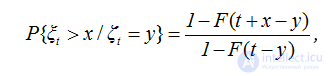
where it is taken into account that there are no renewals on the period [y,t).

Then by the formula of total probability we obtain

or for the distribution function we obtain

(2.41)

From (2.41) we obtain an expression for the expectation

(2.42)

Here it is appropriate to give an expression for the expectation of the interval covering the point t. From equalities (2.40) and (2.42) we obtain the sum

(2.43)

Let us note one important circumstance - the expectation of this interval does not coincide with the expectation of the random variable ξ_.

4. Joint distribution of the forward and backward recurrence times

For 0<=x<=t, y>=0 we write out the probabilities P{ξ_t>=y,η_t>=x}, from which it is easy to obtain the joint distribution P{ξ_tη_t. Indeed,

P{ξ_t>=y,η_t>=x}+P{ξ_tη_tξ_t>=y,η_tξ_tη_t>=x}=1

P{ξ_tξ_tη_tξ_tη_t>=x},

P{η_tξ_tη_tξ_t>=y,η_t

P{ξ_t>=y,η_t>=x}+P{ξ_tη_tξ_tη_t

For the event {ξ_t>=y}⋂{(η_t>=x} to occur, it is necessary and sufficient that there be no renewals on the interval (t-x,t+y). Therefore,

(2.44)

Since the random variable η_t has a positive atom at x=t, we must single out separately the case

P{ξ_t>=y,η_t=t}=1-F(t+y),

which corresponds to the first term in (2.44).

Finally, for x>t, y>=0 the joint probability equals zero by virtue of equality (2.42).

Equality (2.44) shows the dependence of the random variables ξ_t and η_t, since the probability cannot be represented as a product of probabilities and .

In conclusion of this section, let us give the distribution of the interval covering an arbitrary epoch t, that is, the distribution of the sum

For x we obtain

(2.45)

For we obtain

(2.46)

See also

• Poisson random measure
• stochastic process
• random walks
• renewal process
• the Cramér–Lundberg model
• empirical measures
• Poisson random measure