
Lecture
Construction of a sequence of independent real-valued random variables having given distribution functions.
Many important processes can be constructed starting from a sequence of independent random elements.
Let us give a number of examples of this kind. Note that constructing a sequence of independent real-valued random variables requires entirely elementary means, as Exercises 2 and 3 show.
Example 1. Let 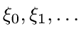 — independent random vectors, defined on some probability space
 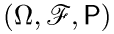 and taking values in the space
 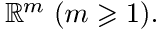 . The random process (with discrete time)
 , (9)
, (9)
is customarily called a random walk.
If we imagine a particle which at the zero time moment is located in the point  and at each (discrete) time moment
 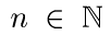 is displaced by
the amount  , then the vector (n,Sn) gives the coordinates of this particle in time and space.
Example 2. For a sequence 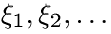 of independent identically distributed nondegenerate nonnegative random variables the renewal process is defined by the formula

Everywhere we take the sum over the empty set to be zero, so that 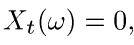 , if
, if 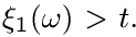 . Generally speaking, the quantities
  so defined take values in
 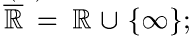 ; here the σ-algebra
  is taken to consist of the sets B and
 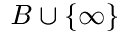 , where
 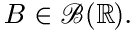 .
.
The name "renewal process" is explained by the following interpretation. Suppose that,
starting from to = 0, at moments separated from one another by intervals  a certain device breaks down (for example, an electric light bulb burns out), and the failed device or its faulty unit is instantly replaced by an identical new one. Then
  is the number of replacements ("renewals") on the interval (0, t]. The trajectory of the process
  is shown in Fig. 2.
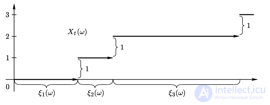
Fig. 2
Example 3. Consider on some probability space 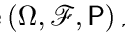 two sequences of nonnegative random variables
such that  are jointly independent and
 . For positive constants y0 and c define the process
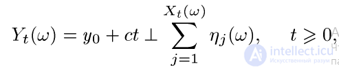
where  is given by formula (10). Processes of the form (11) are used in the Cramer-Lundberg model of insurance, in which y0 —
is the initial capital of the company, c is the rate of premium income,  — the size of the payout at the random moment
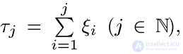 , a Yt is interpreted as the company's capital at time t.
Example 4. Let 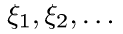 — independent identically distributed random vectors, defined on the probability space
 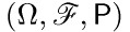 and taking values in
 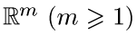 .
.
Let us introduce the empirical measures
 (12)
(12)
Using Definition 3, it is easy to see that formula (12), for each 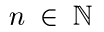 , defines a random process indexed by Borel sets B, i.e.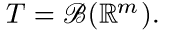
Instead of the indicator 1B in (12) one could take a function f from some class  . Then, given suitable measurability of f, one obtains a random process indexed by a family of functions.
Example 5. Let 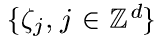 — a random field formed by independent identically distributed vectors with values in
 Let μ be a σ-finite measure* on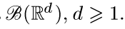
Let us define the process of partial sums
 (13)
(13)
where  is the unit cube with upper vertex
at the point  .
.
In other words, unlike (9), here weighted partial sums of a certain kind are taken.
note
*μ is a σ-finite measure on  if
if 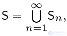 where
where 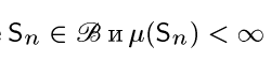 for any

Example 6. Let λ be a finite measure (λ  0), defined on some measurable space
. Let Y, X1, X2,... — independent random elements on the probability space 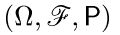 such that Y — a real-valued Poisson variable with parameter
  , a X1, X2,... — independent identically distributed variables that are
  measurable, for which
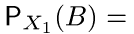
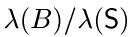 as
as 
. The possibility of such a construction follows from Theorem 2. (Note that here we are dealing with the quantities Y and Xk with values in
different spaces.) Let us introduce on  a function
 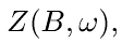 by setting
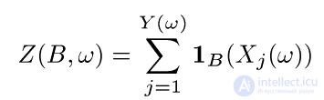 (14)
(14)
(  , when
 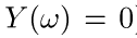 ). Formula (14) defines the so-called Poisson random measure with intensity measure (or governing measure) λ. The case of a σ-finite measure λ is discussed in the supplement to this chapter.
Exercise 2
Let 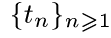 — a sequence of positive numbers such that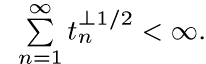
. Prove that then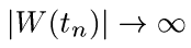 a.s. as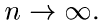
In addition to the local law of the iterated logarithm (see Corollary 3), let us formulate the following useful result on the local behavior of trajectories of the Wiener process.
Exercise 3. Consider a sequence 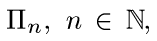 , of refining partitions
  of the segment [0, t] by points of a special form

Then

Let us proceed directly to describing an explicit construction of the Wiener process (on the segment [0,1]) by means of a sequence of independent standard
Gaussian variables.
Theorem 8. Let 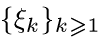 — a sequence of independent random variables, having the standard normal distribution
  and defined on some probability space
 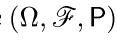 .
.
Let us set for 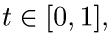

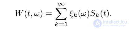
Then  is a Wiener process on [0,1], moreover having, with probability one, continuous trajectories.


Comments