
Lecture
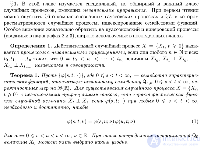

§1. This chapter studies a special but extensive and important class
of random processes having independent increments. On a first reading
one may skip § b on complex-valued Gaussian processes and § 7, in which
random processes indexed by families of functions are considered.
Special attention should be paid to the Poisson and Wiener processes
(introduced in Sections 2 and 3), which are widely used in subsequent chapters.
Definition 1. A real-valued random process X = {Xt, t ^ 0} is called
a process with independent increments if for any n E N and all
to, t\,..., tn such that 0 = to < ti < • • • < tn, the quantities Xto, Xtl _L Xto, ...,
Xtn -L Xtn_1 are independent in the aggregate.
Theorem 1. Let {p(s,t; •)}, where 0 ^ s < t < oo, — be a family of characteris-
tic functions, corresponding to some family Qs,t, 0 ^ s < t < oo, of proba-
bility measures on N§(E). For the existence of a random process X = {Xt,
t ^ 0} with independent increments such that the characteristic func-
tion of the random variable Xt _L Xs is (f(s,t; •) for any 0 ^ s < t < oo,
it is necessary and sufficient that
f, t; v) =
for all 0^s the value of Xq may be chosen arbitrarily.
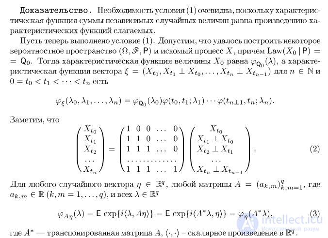
Proof. The necessity of condition A) is obvious, since the characteris-
tic function of the sum of independent random variables equals the product of the cha-
racteristic functions of the summands.
Suppose now that condition A) holds. Assume that we have managed to construct some
probability space (P, ^, P) and the sought process X, with Law(Xo | P) =
= Qo- Then the characteristic function of the value Xo equals aracteristic function of the vector f = (Xto,Xtl -L Xto,..., Xtn -L Xtn_1) for n e N and
0 = to < h < • • • < tn is
i,..., Xn) =
Note that
xtl
Xt2
/10 0
1 1 0
111
0
0
X
\1 1 1
1/
t0
xt
tn-1'
For any random vector r/ G
ak,t ? M (fc,m = 1,..., q), and all A E
, any matrix A =
= E exp{r(L, Ar,)} = E exp{i{A*X,r1)} = ^(
B)
J>m=1, where
C)
where A* — is the transpose of the matrix A, (•,•)- is the inner product in Rq.
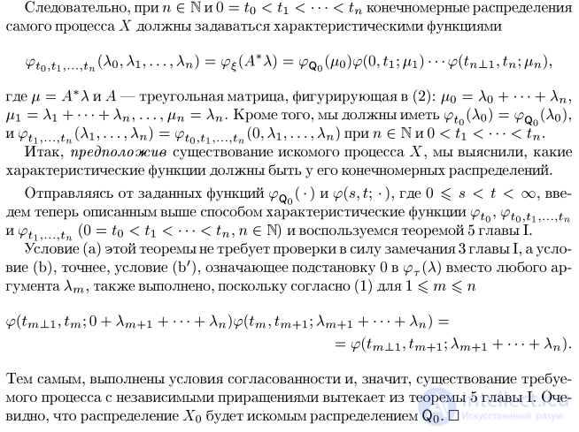
Consequently, for nGNnO = to
where \i — A*Xw A — is the triangular matrix appearing in B): /io = Ao + • • • + An,
A*i = Ai H h An, ..., \in — Xn. In addition, we must have M(Pti,...,tn(Ab---5An) =^to5tb...5tn@,Ai,...,An)npHn G NhO < h < ••• < tn.
Thus, assuming the existence of the sought process X, we have established which
characteristic functions its finite-dimensional distributions must have.
Starting from the given functions ^qo( •) and cp(s, t\ •), where 0 ^ s < t < oo, intro-
duce now, in the manner described above, the characteristic functions iptQ, (Pto,ti,...,tn
and ^tb...,tn @ = ^o < t\ < • • • < tn, n G N) and let us use Theorem 5 of Chapter I.
Condition (a) of this theorem requires no verification by virtue of Remark 3 of Chapter I, while condi-
tion (b), or more precisely, condition (V), meaning the substitution of 0 in <pT(X) in place of any ar-
gument Am, is also satisfied, since according to A) for 1 ^ m ^ n
; 0
An) =
An).
Thus, the consistency conditions are satisfied and, hence, the existence of the requi-
red process with independent increments follows from Theorem 5 of Chapter I. Evi-
dently, the distribution of Xq will be the sought distribution Qq. ?
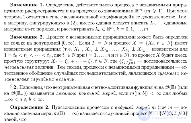
Remark 1. The definition of a real-valued process with independent incre-
ments extends also to processes with values in Mm (m ^ 1). In this case
Theorem 1 remains valid with a minor modification in its proof. Thus,
in the matrix appearing in B), instead of ones one should write 1m — the identity
matrices of order m, and consider A& E Mm, k = 0,1,..., m.
Remark 2. A process with independent increments may be defined
not only on the half-line [0, oo). If T = N and the process X = {Xt, t G N} has
independent increments (i.e., Xt0, Xtx -L Xt0, ..., Xtn -L Xtn_1 are independent for
1 = to < t\ < • • • < tn, where ti G N for i = l,...,nnnGN), then the process X will have
a simple structure: Xt = ?i + • • • + ?t? t ? N, where {^j}'j^1 — is a sequence
of independent random variables. Thus, processes with independent increments are a na-
tural generalization of random sequences that are sums of in-
dependent random variables.
§ 2. Recall that a nonnegative countably additive function m on Ze(R) (or
on N§(M_|_)) is called a locally finite measure if m([a,b]) < oo for all
_Loo < a ^ b < oo.
Definition 2. By a Poisson process with governing measure m (where m — is a lo-
cally finite measure, m(E) = oo) is meant a random process TV = {N(t),t ^ 0}
such that
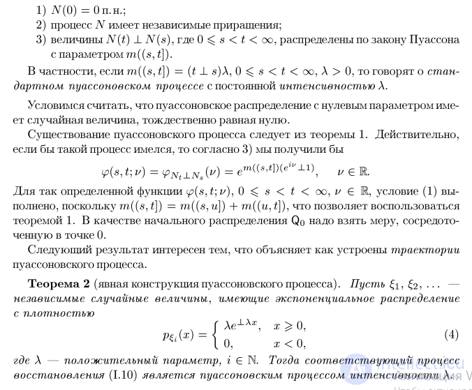
1) jV@) = 0 a.s.;
2) the process N has independent increments;
3) the quantities N(t) _L N(s), where 0 ^ s < t < oo, are distributed according to the Poisson law
with parameter m((s,t]).
In particular, if m((s, i\) = (t _L s)A, 0 ^ s < t < oo, A > 0, then one speaks of the stan-
dard Poisson process with constant intensity A.
Let us agree that a Poisson distribution with zero parameter is possessed by the ran-
dom variable that is identically equal to zero.
The existence of the Poisson process follows from Theorem 1. Indeed,
if such a process existed, then according to 3) we would obtain
f,Uu) =
Theorem 1. As the initial distribution Qo one should take the measure concen-
trated at the point 0.
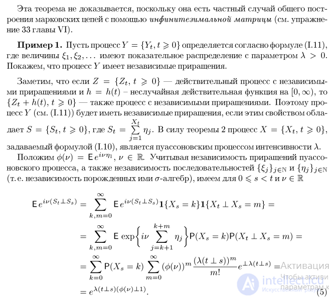
The following result is of interest in that it explains how the trajectories
of the Poisson process are structured.
Theorem 2 (explicit construction of the Poisson process). Let ?i, ?2 ? • • • —
be independent random variables having an exponential distribution
with density
^ x > 0,
x<0, D)
where A — is a positive parameter, r G N. Then the corresponding process
of renewal A.10) is a Poisson process of intensity A.
This theorem is not proved, since it is a particular case of the general construc-
tion of Markov chains by means of an infinitesimal matrix (see Exer-
cise 33 of Chapter VI).
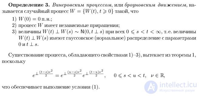
Example 1. Let the process Y = [Yt,t ^ 0} be defined according to formula A.11),
where the quantities ?i, ?2? • • • have an exponential distribution with parameter L > 0.
Let us show that the process Y has independent increments.
Note that if Z = {Zt, t ^ 0} — is a real-valued process with independ-
ent increments, and h = h(t) — is a non-random real-valued function on [0, oo), then
{Zt + h(t), t ^ 0} — is also a process with independent increments. Therefore the pro-
cess Y (see A.11)) will have independent increments if this property is posses-
xt
sed by S = {St, t ^ 0}, where St = Yl Vj- By virtue of Theorem 2 the process X = {Xt, t ^ 0},
given by formula A.10), is a Poisson process of intensity L.
Let us set f(y) = E elvril, v G E. Taking into account the independence of the increments of the Pois-
son process, as well as the independence of the sequences {?j}j^n and {
(i.e., the independence of the sigma-algebras generated by them), we have for 0^s k,m=0
oo
k,m=O
oo oo / l / j I \ \
V P(X =k)Y^ (fA'))sh^ ^
k=0 m=0
Vj\P(Xs=k)P(Xt±Xs=m) =
Similarly one computes the joint characteristic function of the set of increm-
ents of the process {St, t ^ 0}, whence the required assertion follows.

Wiener process in the theory of random processes is a mathematical model of Brownian motion or a random walk with continuous time.
A random process  , where
  is called a Wiener process if
 almost surely. — is a process with independent increments.
 ,
,  ,
,where 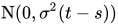 – is the normal distribution with mean
  and variance
  . The quantity
  , constant for the process, will henceforth be taken equal to
  .
.
An equivalent definition:
– is a Gaussian process. ,
,  .
. ,
,  .
.There exists a unique Wiener process such that almost all of its trajectories are everywhere continuous. Since it is usually this process that is considered, the condition of continuity of the trajectories is often included in the definition of the Wiener process.
— is a Gaussian process. — is a Markov process.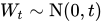 . Accordingly,
  and
and  .
. . - is a martingale. Here by a martingale we mean
  — is a Wiener process, then
  and
and  , will also be Wiener. — is a Wiener process, and
  , then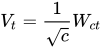
is also a Wiener process.
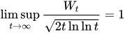 almost surely.
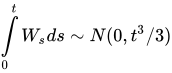
A multidimensional ( -dimensional) Wiener process
  — is an
  -valued random process composed of independent one-dimensional Wiener processes, that is
 ,
,
where the processes  are jointly independent.
The Wiener process describes the Brownian motion of a particle undergoing disordered movements under the influence of impacts from liquid molecules. The constant here depends on the mass of the particle and the viscosity of the liquid.
The Poisson process, Poisson flow, Poisson stream — is an ordinary flow of homogeneous events, for which the number of events in the interval A does not depend on the numbers of events in any intervals not intersecting with A, and obeys the Poisson distribution. In the theory of random processes it describes the number of random events that have occurred, occurring with constant intensity.
The probabilistic properties of a Poisson flow are completely characterized by the function Λ(A), equal to the increment on the interval A of some decreasing function. Most often the Poisson flow has an instantaneous value of the parameter λ(t) — a function, at whose points of continuity the probability of a flow event in the interval [t,t+dt] equals λ(t)dt. If A — is the segment [a,b], then
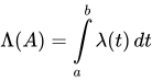
A Poisson flow for which λ(t) equals the constant λ is called the simplest flow with parameter λ.
Poisson flows are defined for a multidimensional space, and in general for any abstract space in which one can introduce a measure Λ(A). A stationary Poisson flow in a multidimensional space is characterized by the spatial density λ. Here Λ(A) equals the volume of the region A multiplied by λ.
Two types of Poisson processes are distinguished: simple (or simply: the Poisson process) and compound (generalized).
Let  . A random process
  is called a homogeneous Poisson process with intensity
  if
if
 almost surely.
 — is a process with independent increments.
 for any
  , where
  denotes the Poisson distribution with parameter
  .
. be a sequence of mutually independent identically distributed random variables.
 — be a simple Poisson process with intensity , independent of the sequence .
Denote by  the sum of the first k elements of the sequence introduced.
Then let us define the compound Poisson process  as
as  .
.
 .
. ,
,
that is, the moment of the  -th jump has a gamma distribution
  .
.


 as
as  ,
,
where  denotes «little o».
In order for some random process with continuous time to be Poisson (simple, homogeneous) or identically zero, it suffices that the following conditions hold:
. as
as  .
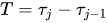
. — be the jump moments of the Poisson process.
  .
.Does  depend on the preceding part of the trajectory?
 — ?
— ?
Let  .
.


 .
.
The distribution of the lengths of the time intervals between jumps has the memoryless property ⇔ it is exponential.
 on the time axis.
 — is the number of jumps on the segment .
The conditional distribution of the jump moments  coincides with the distribution of the order statistics constructed from a sample of size from
  .
.
The density of this distribution 

Rate of convergence:
 ,
,
where  — is the Berry-Esseen constant.
The Poisson flow serves to model various real flows: accidents, the flow of charged particles from space, equipment failures, and others. It is also possible to apply it to the analysis of financial mechanisms, such as a flow of payments and other real flows, as well as for constructing models of various queueing systems and analyzing their suitability.
The use of Poisson flows considerably simplifies the solution of queueing-system problems related to computing their efficiency. But an unjustified replacement of a real flow by a Poisson flow, where this is not admissible, leads to gross miscalculations.
§ 3. Let us introduce one of the most important random processes.
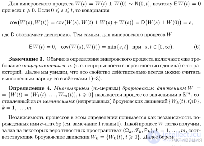
Definition 3. By a Wiener process, or Brownian motion, is me-
ant a random process W = {W(t), t ^ 0} such that
1) W@) = 0 a.s.;
2) the process W has independent increments;
3) the quantities W(t) _L W(s) ~ N@, t _L s) for all 0 ^ s < t < 00, i.e., the quantities
W(t) _L W(s) have a Gaussian (normal) distribution with parameters
The existence of a process possessing properties 1)-3) follows from Theorem 1,
since
, (t-s)u2 , (u-s)u2 , (t-u)u2
e^ 2 = e^ 2 e^ 2 , 0 ^ s < u < ?, v G E,
which ensures that condition A) holds.
50 A. V. Bulinsky, A. N. Shiryaev
For the Wiener process W(t) = W(t) _L W@) ~ N@,?), therefore EW(t) = 0
for all t ^ 0. If 0 ^ s ^ ?, then the covariance
cov(W(s), W(t)) = cov(W(s), W(?) _L W(s) + W(s)) = D(W(s) _L W@)) = 5,
where D denotes the variance. Thus, for the Wiener process W
EW(t)=0, cov(W(s),W(t)) = min{s,?} for s,t e[0,oo). F)
Remark 3. Usually the definition of the Wiener process also includes the re-
quirement of continuity a.s. (i.e., continuity with probability one) of its tra-
jectories. Further on we shall see that this property can indeed always be regarded as
holding along with properties 1)-3).
Definition 4. By a multidimensional (m-dimensional) Brownian motion W =
= {W(?) = (Wi(t),..., Wm(t)), t ^ 0} is meant a process with values in Em, com-
posed of m independent (continuous) Brownian motions {Wk(t), t^O},
k = 1,... ,?mr.
Independence of the processes in this definition is understood as the independence of the gen-
erated sigma-algebras (see Remark 1 of Chapter I). Such a process W is easily obtained,
by specifying on certain probability spaces (P&, ^, P&), k = 1,..., m, corres-
ponding Brownian motions Wk = {Wk(t), t ^ 0}. Next we take
k=1
and extend the definition of Wk on P analogously to formula A.46).

Comments