. Construction of Brownian motion from Schauder functions and a sequence of independent Gaussian random variables: a) two lemmas; b) construction on [0,1]; c) construction on [0,¥].
Definition of Brownian motion and its existence
One of the most important random processes is the Wiener process, also called Brownian motion.
Definition 4.1. A random process {W(t), t > 0} is called standard Brownian motion if
1) W(0) = 0 a.s.;
2) the increments of the process W(t1), W(t2) − W(t1), . . . , W(tm) − W(tm−1) for any m ∈ N and t1, t2, . . . , tm such that 0 < t1 < t2 < · · · < tm, are independent random variables;
3) the random variable W(t) − W(s) has a normal distribution with parameters 0 and t − s for any t, s such that
0 6 s < t;
4) the trajectories of the process {W(t)} are a.s. continuous.
Another definition of Brownian motion can also be given.
Definition 4.2. A random process {W(t), t > 0} is called standard Brownian motion if
1) W(0) = 0 a.s.;
2) the random vector {W(t1), W(t2), . . . , W(tm)} has a multivariate normal distribution for any m ∈ N and
t1, t2, . . . , tm such that 0 < t1 < t2 < · · · < tm;
3) EW(t) = 0 for any t ∈ [0,∞), cov (W(t1), W(t2)) = min (t1, t2) for any t1, t2 ∈ [0,∞);
4) the trajectories of the process {W(t)} are a.s. continuous.
Before proving the equivalence of these definitions,
let us recall some facts about normal distributions. A random variable ξ is said to have a normal distribution
with parameters a ∈ R and σ
2 ∈ (0,∞) (notation: ξ ∼ Na, σ2),
if ξ is a continuous random variable with density
of probability
The normal distribution is called standard if a = 0,σ2 = 1. In this case the distribution function is denoted Φ(x)
and is called the Laplace function
Let ξ1, ξ2, . . . , ξn – independent random variables and ξi ∼
N(0, 1) for i = 1, 2, . . . , n. Consider the random vector ξ =
{ξ1, ξ2, . . . , ξn}. Let A and b – arbitrary numerical matrices
of size n×n and n×1. The distributions of the random vectors Aξ +b
(here the random vectors are represented as columns), and only these, are called n-dimensional normal distributions.
Random vectors with such distributions are called normal.
If {η1, η2, . . . , ηn} – a normal vector and cov (ηi
, ηj ) = 0 for
all i, j such that i 6= j, then the random variables η1, η2, . . . , ηn are independent. If, however, cov (ηi
, ηj ) = 0 for all i, j such that,
i 6 k, j > k for some k ∈ {1, 2, . . . , n − 1}, then the random
vectors {η1, η2, . . . , ηk} and {ηk+1, ηk+2, . . . , ηn} are independent.
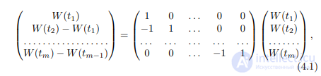
Proof of equivalence. Obviously,
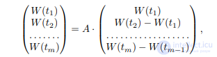
, (4.2)
where A – is the matrix inverse to the first matrix on the right-hand side of (4.1).
If W satisfies the conditions of Definition 1, then the random vector {W(t1), W(t2) − W(t1), . . . , W(tm) − W(tm−1)} is normal, whence, in view of (4.2), the random vector
{W(t1), W(t2), . . . , W(tm)} is also normal. Further, for t2 > t1
(here it is taken into account that W(t1) and (W(t2) − W(t1)) – are independent random variables, and therefore EW(t1) (W(t2) − W(t1)) = 0).
If, on the other hand, W satisfies the conditions of Definition 4.2, then, in view of (4.1), from the fact that the vector {W(t1), W(t2), . . . , W(tm)} is normal, it follows that the vector {W(t1), W(t2) − W(t1), . . . ,
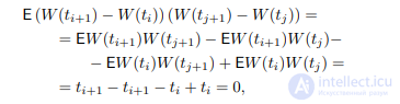
W(tm)−W(tm−1)} is normal. Its components are uncorrelated, since for j > i
therefore the random variables W(t1), W(t2) − W(t1), . . . , W(tm) − W(tm−1) are independent. Finally,
The equivalence is proved.
Let us prove the existence of Brownian motion. We give its explicit construction, based on a sequence of independent random variables with the same distribution N(0, 1) and the Schauder functions.
Let us give their definition, but first let us recall the definition
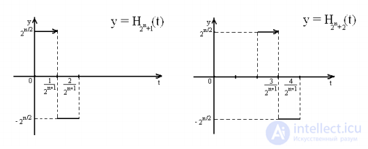
of the Haar functions. These functions are denoted Hi(t), i ∈ N, and are defined on the interval [0, 1]. The function H1 is identically equal to 1. For
each n ∈ N0 (N0 = {0, 1, 2, . . . }) let us introduce 2
n Haar functions
H2n+k, where k = 1, 2, . . . , 2
n. For this purpose we divide the interval [0, 1] into 2 n equal subintervals and number them from left to right. Take the k-th such subinterval. Outside it we set H2n+k(t) = 0. Divide the given subinterval in half. On its left half we set H2n+k(t) = 2−n/2
, and on the right half we set H2n+k(t) = −2−n/2 (see fig. 2).
Consider the space L2[0, 1] of measurable numerical functions x, defined on the interval [0, 1] and square-integrable:

It is known that the Haar functions form a complete orthonormal system in the space L
2[0, 1] with the inner product
Fig. 2.
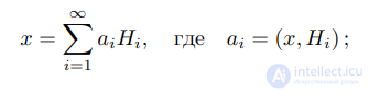
Therefore any function x ∈ L2[0, 1] can be expanded in a series with respect to
this system of functions:
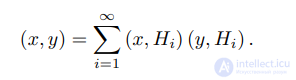
and Parseval's equality holds:
Let us construct continuous nonnegative functions Si(t), called the Schauder functions, based on Hi(t):
Si(t) = Z t0Hi(s) ds, i ∈ N.
Obviously, for i ∈
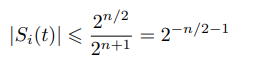
(4.3)
and for different

the functions Si1 (t), Si2
(t) have disjoint supports.
Let us establish two auxiliary statements.
Lemma 4.1. Let a numerical sequence {ai, i ∈ N} be such that ai = O (iε) as i → ∞ for some ε ∈ (0, 1/2).
Then the series
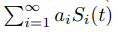
converges uniformly in t on the interval [0, 1].
Proof. There exists a positive constant K such that for all i ∈ N the inequality
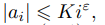
holds
,
therefore for all

.
Hence, taking into account (4.3) and the fact that the functions Si(t) for different
have pairwise disjoint supports, we obtain that for all t ∈ [0, 1]
.
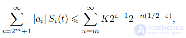
Consequently, for m ∈ N0, t ∈ [0, 1]
,
but the right-hand side tends to zero as m → ∞. The lemma is proved.
Lemma 4.2. Let ξ1, ξ2, . . . – random variables defined on the same probability space (Ω, F, P), with
ξi ∼ N(0, 1), i ∈ N. Then for an arbitrary constant c ∈
√
2,∞
and for almost every (a.e.) ω ∈ Ω there exists a natural number N0 (c, ω) such that for all i > N0 (c, ω) we have |ξi
| < c√
ln i.
Proof. We shall need the Borel–Cantelli lemma, which states that if random events A1, A2, . . . are such that P∞
i=1 P (Ai) < +∞, then for a.e. ω only a finite number of the events A1, A2, . . . occur. Note that if ξ ∼ N(0, 1),
then for x > 0

. (4.4)
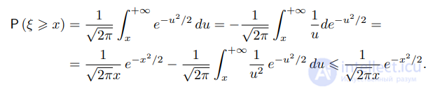
Indeed,
.
Therefore for i > 2
For c > √2 the series
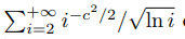
converges. Consequently, for
a.e. ω the inequality |ξi(ω)| > c
√
ln i holds only for i in a finite set. The lemma is proved.
Theorem 4.1. Let ξ1, ξ2, . . . – independent random variables, with ξi ∼ N(0, 1), i ∈ N; S1,S2, . . . – the Schauder functions,
then
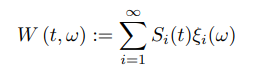
(4.5)
is Brownian motion for t ∈ [0, 1].
Proof. By Lemmas 4.1 and 4.2, for a.e. ω the series on the right-hand side of (4.5) converges uniformly in t on the interval [0, 1]. The functions Si(t) are continuous in t for any i ∈ N. Consequently, for
a.e. ω the right-hand side of (4.5) is a continuous function of t.
Let us show that the series on the right-hand side of (4.5) converges in mean
square. Recall that if η, η1, η2, . . . – random variables defined on the same probability space, then convergence in mean square of the random sequence {ηn} to η as n → ∞ (notation: ηn
m.s. → η) means that
limn→∞ E (ηn − η)
2 = 0; the random sequence {ηn} converges in mean square as n → ∞ if and only if,
E (ηm − ηl)
2 → 0 as m, l → ∞. Similarly the notion of mean-square convergence is introduced for a sequence of random vectors. For m > l we have that
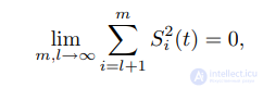
Recalling the properties of the Schauder functions, we see that
Consequently,
which is the required mean-square convergence.
Since both a.s. convergence and mean-square convergence imply convergence in probability, the limits of the right-hand side of (4.5) in both cases are equal a.s.
Let us show the validity of properties 1), 2), 3) of Definition 4.2
of Brownian motion.
1) Since Si(0) = 0 for all i ∈ N, we have W(0) = 0 a.s.
2) The mean-square limit of a sequence of normal random vectors is a normal random
vector. Since for m ∈ N and t1, . . . , tm ∈ (0, 1] as n → ∞

(4.6)
and the vector on the left is normal, the vector on the right is also
normal.
3) From relation (4.6) it follows that the expectations
and covariances of the components of the random vector on the left-hand
side converge, so as n → ∞
a)

, but the left-hand side equals zero, hence EW(t) = 0 for any t ∈ [0, 1];
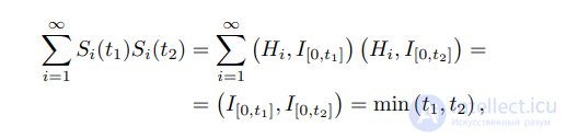
b)

but the left-hand side equals Pn
i=1 Si(t1)Si(t2) and its limit equals (recall Parseval's equality)
hence, EW(t1)W(t2) = min (t1, t2) for t1, t2 ∈ [0, 1] (here
I[a,b] (·) – is the indicator of the interval [a, b]).
The theorem is proved.
Remark 4.1. Using the completion procedure for the probability space on which the random variables ξ1, ξ2, . . . are defined, and setting W (t, ω) = 0 for t ∈ [0, 1] and those ω for which the series on the right-hand side of (4.5) does not converge uniformly in t on the interval [0, 1], we obtain Brownian motion all of whose trajectories are
continuous. In what follows we shall consider precisely such Brownian mot
Finally, let us discuss the construction of Brownian motion for all t ∈ [0,∞). For this purpose consider a sequence of independent Brownian motions W1, W2, . . . , defined for t ∈ [0, 1], and set W(t) = W1(t) for t ∈ [0, 1],
W(t) = W1(1) + W2 (t − 1) for t ∈ [1, 2], W(t) = W1(1) + W2(1) + W3 (t − 2) for t ∈ [2, 3], and so on. The resulting process W is Brownian motion on the half-line [0,∞) (the proof is left to the reader). In connection with this construction it is appropriate to mention the so-called Markov property
of Brownian motion W: for each t0 ∈ (0, +∞) the random process {W (t0 + t) − W(t0), t ∈ [0, +∞)} is Brownian motion, independent of the past, i.e., of the process {W(t), t ∈ [0, t0]}.
The construction of Brownian motion indexed by sets, using Haar functions, is carried out in the work
Ruke R. The Haar-function constraction of Brownian motion indexed by sets // Z. Wahr. verw. Geb. - 1983. - Bd. 64, H. 4. - S. 523-539.











Comments