
Lecture
Monte Carlo methods (MCM) — a group of numerical methods for studying random processes. The essence of the method is as follows: the process is described by a mathematical model using a random-number generator, the model is computed repeatedly, and the probabilistic characteristics of the process under consideration are calculated from the data obtained. For example, to find out by the Monte Carlo method what the average distance will be between two random points in a circle, one needs to take the coordinates of a large number of random pairs of points within the boundaries of a given circle, compute the distance for each pair, and then calculate the arithmetic mean of them.
The methods are used to solve problems in various fields of physics, chemistry, mathematics, economics, optimization, control theory and others.
The name of the method comes from the Monte Carlo district, known for its casinos.
The Monte Carlo method has many different applications. It is used in the following areas: in industry, for modeling the variability of production processes; in physics, chemistry and biology, for modeling various phenomena; in games, for modeling artificial intelligence, for example in the Chinese game of Go; in finance, for valuing derivative financial instruments and options. In essence, the Monte Carlo method is used everywhere.
The modern version of the method was formed within the framework of the Manhattan Project, where it was used to model the distances that neutrons could travel through various materials. The idea of modeling based on generating a set of random values had already existed for some time, but received particular development during the creation of the atomic bomb, subsequently spreading to many other fields of knowledge.
A major advantage of the Monte Carlo method is that it allows an element of randomness and the complexity of the real world to be taken into account in the model. Moreover, the method is robust with respect to changes in various parameters, such as the distribution of the random variable. It is based on the law of large numbers.
One of the typical examples of using the Monte Carlo method is problems in which it is necessary to find the mathematical expectation of some random variable. To do this, one needs to generate a set of random values of this variable and find the mean. The random variable is usually characterized by a certain probability distribution.
The essence of the method is as follows: for the target random variable a set of random values is generated, and then the required values are calculated on its basis.
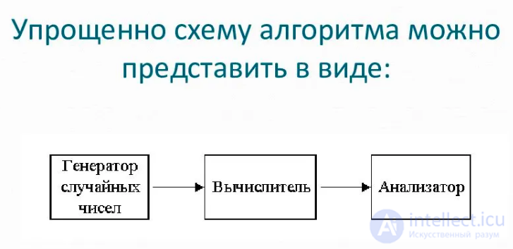
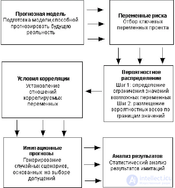
The essence of the Monte Carlo method is as follows: it is required to find the value A of some quantity under study. To do this, a random variable X is chosen whose mathematical expectation equals A: M(X) = A. In practice, one proceeds as follows: N trials are performed, yielding N possible values of X, their arithmetic mean is computed, and it is taken as an estimate (approximate value) A ’ of the sought number A. As a rule, a program is written to carry out a single random trial. The computational error is, as a rule, proportional to D/ sqrt (N), where D – is some constant. This means that N must be large, so the method relies heavily on computing power. It is clear that achieving high precision this way is impossible. This is one of the drawbacks of the method. In many problems it is possible to significantly increase precision by choosing a calculation approach corresponding to a significantly smaller D.
Unlike analytical methods, which seek a solution in the form of a series in eigenfunctions, Monte Carlo methods seek solutions in the form of statistical sums. To apply them, a description of the probabilistic process suffices, and its formulation as an integral equation is not required; the error estimate is extremely simple, and their accuracy depends only weakly on the dimensionality of the space. I confirmed this myself by running experiments to solve two simple problems. The results of the experiments demonstrated their accuracy, which is why the Monte Carlo method is used to solve many complex problems that are very difficult or impossible to solve by other methods
Random variables have been used to solve various applied problems for quite a long time. An example is the method for determining the number Pi proposed by Buffon back in 1777. The essence of the method was to drop a needle of length  onto a plane ruled with parallel lines spaced
  apart from one another (see Fig. 1).

The probability (as is clear from the further context, this is not actually a probability but the mathematical expectation of the number of intersections per trial; it becomes a probability only under the condition  ) that the segment will cross a line is related to the number Pi:
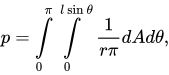
where
 — the distance from the end of the needle to the nearest line;
 — the angle of the needle relative to the lines.
This integral is easy to evaluate:  (provided that ), so by counting the proportion of segments that cross the lines, one can approximately determine this number. As the number of trials increases, the accuracy of the result obtained will increase.
In 1864, Captain Fox, recovering from a wound and looking for a way to occupy himself, carried out the needle-dropping experiment . The results are presented in the following table:
| Number of throws | Number of intersections | Needle length | Distance between lines | Rotation | Value of Pi | Error | |
|---|---|---|---|---|---|---|---|
| First attempt | 500 | 236 | 3 | 4 | none | 3.1780 | +3,6⋅10-2 |
| Second attempt | 530 | 253 | 3 | 4 | present | 3.1423 | +7,0⋅10-4 |
| Third attempt | 590 | 939 | 5 | 2 | present | 3.1416 | +4,7⋅10-5 |
Comments:
The number Pi can be calculated using the Monte Carlo method.
By inscribing a circle in a square (the diameter of the circle equals the side of the square), the ratio of the area of the circle to the area of the square can be expressed as follows:
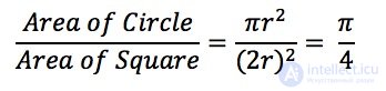
If we can calculate this ratio, then we can obtain the value of the number Pi.
Let us fill the square with points having random coordinates. We calculate the ratio of the number of points that fall inside the circle to the total number of points. We multiply the result by 4 to obtain the value of the number Pi.
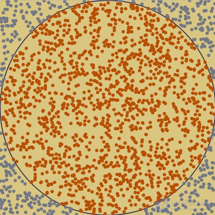
The greater the number of points, the closer the obtained value is to the true value of the number Pi.
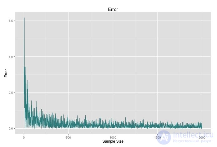
This simple example demonstrates the Monte Carlo method in action.
example in the R language
|
# estimating pi using Monte Carlo methods. This code won't run perfectly for you, because I # didn't save everything I did, like adding vectors to a dataframe named Pi. |
|
| # Just the important stuff is here. | |
| center <- c(2.5, 2.5) # the center of the circle | |
| radius <- 2.5 | |
| distanceFromCenter <- function(a) { | |
| sqrt(sum((center - a) ^ 2)) | |
| } | |
| # let's define a 5 by 5 square matrix | |
| points <- c(0,0, 0,5, 5,5, 5,0) | |
| square <- matrix(points, nrow = 4, ncol = 2, byrow = TRUE) | |
| # now all I need to do is make matrix A a matrix of real simulated points. | |
| n <- 100 # number of points | |
| A <- matrix(runif(n*2, min=0, max=5), nrow = n, ncol = 2, byrow = T) # random sampling occurs here!!! | |
| ## An alternate way to generate randoms, with faster convergence | |
| # library(randtoolbox) | |
| # A <- matrix(5*halton(n*2), nrow = n, ncol = 2, byrow = T) | |
| # here's how you'll test if it's in the circle. | |
| b <- apply(A, 1, distanceFromCenter) | |
| # d <- subset(b, b < radius) # if you know a better way to do this part, email me. | |
| # num <- length(d) / length(b) | |
| num <- mean(b < radius) | |
| piVec <- c() | |
| for (i in 1:2000) { | |
| n <- i | |
| A <- matrix(runif(n*2, min=0, max=5), nrow = n, ncol = 2, byrow = T) | |
| b <- apply(A, 1, distanceFromCenter) | |
| d <- subset(b, b < radius) | |
| num <- length(d) / length(b) | |
| piVec[i] = num*4 | |
| } | |
| library(data.table) | |
| Pi <- data.frame(piVec) | |
| Pi <- data.table(Pi) | |
| Pi[, ind := seq(0, 1999)] | |
| Pi[, error := abs(pi - piVec)] | |
| Pi <- data.frame(Pi) | |
| names(Pi) <- c("guess", "ind", "error") | |
| ##### Graphing the error | |
| # note - if you want this part to work for you, you'll have to create the appropriate data frame from the piVec vector. | |
| library(ggplot2) | |
| ggplot(Pi, aes(x = ind, y = error)) + | |
| geom_line(colour = '#388E8E') + | |
| ggtitle("Error") + | |
| xlab("Sample Size") + | |
| ylab("Error") | |
The development of the mathematical apparatus of stochastic methods began at the end of the 19th century. In 1899, Lord Rayleigh showed that a one-dimensional random walk on an infinite lattice can give an approximate solution to one type of parabolic differential equation . Andrey Nikolaevich Kolmogorov, in 1931, gave a great impetus to the development of stochastic approaches to solving various mathematical problems, since he succeeded in proving that Markov chains are connected with certain integro-differential equations. In 1933, Ivan Georgievich Petrovsky showed that a random walk forming a Markov chain is asymptotically related to the solution of an elliptic partial differential equation. After these discoveries it became clear that stochastic processes can be described by differential equations and, accordingly, studied using the mathematical methods, well developed by that time, for solving such equations.
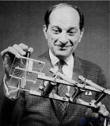
First Enrico Fermi in the 1930s in Italy, and then John von Neumann and Stanislaw Ulam in the 1940s in Los Alamos, suggested that the connection between stochastic processes and differential equations could be used «in reverse». They proposed using a stochastic approach to approximate multidimensional integrals in the transport equations that arise in connection with the problem of neutron motion in an isotropic medium.
The idea was developed by Ulam who, while playing solitaire during his recovery from an illness, wondered what the probability was that the solitaire game would come out. Instead of using the combinatorial reasoning usual for such problems, Ulam suggested that one could simply run the experiment a large number of times and, by counting the number of successful outcomes, estimate the probability. However, because of the need to carry out a large number of repetitive experimental actions, the method did not become widespread.
With the advent of the first electronic computer, ENIAC, which could generate pseudorandom numbers at high speed and use them in mathematical models, interest in stochastic methods was revived. Stanislaw Ulam discussed his ideas with John von Neumann, who ultimately used ENIAC for the statistical-sampling method proposed by Ulam in solving various neutron-transport problems . Due to the need to shut down ENIAC for a significant time at the end of 1946, in order to continue research into neutron transport, Enrico Fermi even designed a specialized analog computer named FERMIAC (by analogy with ENIAC, but indicating Fermi's authorship), which also implemented the Monte Carlo method at the mechanical level.
After computers came into use, a major breakthrough occurred, and the Monte Carlo method was applied to many problems for which the stochastic approach proved more effective than other mathematical methods. Nevertheless, the use of this technique also had its limitations, owing to the need for a very large number of computations to obtain results with high accuracy.
The year of birth of the term «Monte Carlo method» is considered to be 1949, when the article by Metropolis and Ulam «The Monte Carlo Method» was published. The name of the method comes from the name of a commune in the Principality of Monaco, widely known for its numerous casinos, since roulette is one of the most widely known generators of random numbers. Stanislaw Ulam writes in his autobiography «Adventures of a Mathematician» that the name was suggested by Nicholas Metropolis in honor of his uncle, who was a gambler.
In the 1950s the method was used for calculations in the development of the hydrogen bomb. The main credit for developing the method during this period belongs to staff at US Air Force laboratories and the RAND Corporation. Among the first to apply the Monte Carlo method to the calculation of particle showers were the Soviet physicists A. A. Varfolomeev and I. A. Svetlolobov .
In the 1970s, in the new field of mathematics — computational complexity theory, it was shown that there exists a class of problems whose complexity (the number of computations required to obtain an exact answer) grows exponentially with the dimensionality of the problem. Sometimes, by sacrificing accuracy, one can find an algorithm whose complexity grows more slowly, but there is a large number of problems for which this cannot be done (for example, the problem of determining the volume of a convex body in n-dimensional Euclidean space), and the Monte Carlo method is the only way to obtain a sufficiently accurate answer in an acceptable amount of time.
At present, the main efforts of researchers are directed toward creating efficient Monte Carlo algorithms for various physical, chemical, and social processes for parallel computing systems.
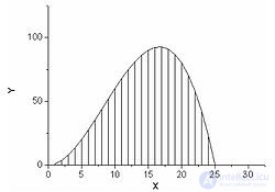
Suppose it is necessary to take the integral of some function. Let us use an informal geometric description of the integral and understand it as the area under the graph of this function.
To determine this area, one can use one of the usual numerical integration methods: divide the segment into subsegments, calculate the area under the function's graph on each of them, and sum them. Suppose that for the function shown in Figure 2, it is sufficient to divide it into 25 segments and, consequently, to compute 25 function values. Now suppose we are dealing with an  -dimensional function. Then we need
  segments and just as many function-value computations. When the dimensionality of the function exceeds 10, the task becomes enormous. Since high-dimensional spaces occur, in particular, in problems of string theory, as well as in many other physical problems involving systems with many degrees of freedom, a solution method is needed whose computational complexity does not depend so strongly on dimensionality. It is precisely this property that the Monte Carlo method possesses.
Suppose it is required to compute a definite integral

Consider a random variable  , uniformly distributed on the interval of integration
  . Then
  will also be a random variable, whose expected value is expressed as
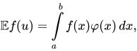
where  — is the probability density of the random variable , equal to
  on the interval . Thus, the desired integral is expressed as
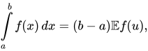
but the expected value of the random variable can easily be estimated by simulating this random variable and computing the sample mean.
So, we throw  points, uniformly distributed over , and for each point
  we compute
  . Then we compute the sample mean:
  . As a result, we obtain an estimate of the integral:
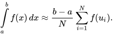
The accuracy of the estimate depends only on the number of points .
This method also has a geometric interpretation. It is very similar to the deterministic method described above, with the difference that instead of uniformly dividing the region of integration into small intervals and summing the areas of the resulting «columns», we scatter random points over the region of integration, and on each of them we build the same kind of «column», defining its width as  , and sum their areas.
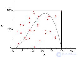
To determine the area under the graph of a function, the following stochastic algorithm can be used:
 can easily be computed; any side of the rectangle touches at least one point of the function's graph, but does not cross it; points), whose coordinates will be chosen at random;
 points) that fall under the graph of the function;
 is given by the expression
For a small number of dimensions of the function being integrated, the performance of Monte Carlo integration is much lower than the performance of deterministic methods. Nevertheless, in some cases, when the function is given implicitly and it is necessary to determine a region defined by complex inequalities, the stochastic method may prove preferable.
With the same number of random points, the accuracy of the computation can be increased by bringing the region bounding the desired function closer to the function itself. To do this, one must use random variables with a distribution whose shape is as close as possible to the shape of the function being integrated. This is the basis of one of the methods for improving convergence in Monte Carlo computations: importance sampling.
Various variations of the Monte Carlo method can be used to solve optimization problems. For example, the simulated annealing algorithm.
Computer simulation plays an important role in modern physics, and the Monte Carlo method is one of the most widespread across many fields, from quantum physics to solid-state physics, plasma physics, and astrophysics.
Traditionally, the Monte Carlo method was used to determine various physical parameters of systems in a state of thermodynamic equilibrium. Suppose there is a set of  possible states of a physical system . To determine the average value
  of some quantity , it is necessary to compute
 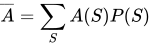 , where the summation is carried out over all states from , and
  — is the probability of state .
Direct simulation by the Monte Carlo method of some physical process involves simulating the behavior of the individual elementary parts of the physical system. In essence, this direct simulation is close to solving the problem from first principles, though for the sake of speeding up computations, the application of certain physical approximations is usually permitted. Examples include calculations of various processes by the method of molecular dynamics: on one hand, the system is described through the behavior of its elementary constituent parts, while on the other hand, the interaction potential used is often empirical.
Examples of direct simulation by the Monte Carlo method:
The quantum Monte Carlo method is widely used to study complex molecules and solids. This name unites several different methods. The first of these is the variational Monte Carlo method, which is essentially the numerical integration of multidimensional integrals arising in the solution of the Schrodinger equation. To solve a problem involving 1000 electrons, one must take 3000-dimensional integrals, and in solving such problems the Monte Carlo method has an enormous performance advantage compared to other numerical integration methods. Another variety of the Monte Carlo method — is the diffusion Monte Carlo method.
Other examples of applications of the Monte Carlo method.
A mathematical description of the characteristics of light propagation can be performed analytically using the Maxwell theory equation or through transport theory. The applicability of Maxwell's equations is limited due to the difficulties involved in deriving exact analytical solutions. On the other hand, the heuristic character of transport theory allows numerical methods to be used to solve the transport of photons through absorbing and scattering media. The Monte Carlo method is widely used to solve problems of radiative transfer because of its flexibility and simplicity in simulating energy transport in arbitrary geometries with complex boundary conditions. Nevertheless, most simulations do not take into account the polarization of light.
statistical methods for simulating electron transport in matter.
Mathematical modeling of the processes of interaction between ionizing radiation and objects of complex geometry and internal structure is of great importance in many applications. In particular, within the framework of problems of X-ray diagnostics of materials and structures, it is necessary to determine and study X-ray images of objects , and when studying the electromagnetic effect of penetrating radiation, it is necessary to analyze the distribution of fluxes of relativistic electrons arising from the interaction of ionizing radiation with the materials of objects. Computational algorithms based on statistical modeling by the Monte Carlo method of the processes of transport and interaction of radiation with matter . The advantage of the Monte Carlo method over alternative methods based on the numerical solution of the kinetic equation is determined by the convenience and suitability of this method for solving complex boundary-value problems in multicomponent media. The effectiveness of applying the Monte Carlo method is currently determined, first, by the development of ways to reduce the statistical error of computation results and, second, by progress in creating high-speed multiprocessor computing systems. Statistical modeling of the transport of electrons and other charged particles presents considerably greater difficulty than modeling the transport of photons.
Monte Carlo N-Particle Transport ( MCNP ) - is a general-purpose continuous-energy, generalized-geometry, time-dependent Monte Carlo radiation transport code, designed for tracking many types of particles over a wide range of energies and developed by Los Alamos National Laboratory . Specific areas of application include, among others, radiation protection and dosimetry, radiation shielding , radiography , medical physics, nuclear criticality safety , detector design and analysis, nuclear well logging for oil wells , accelerator target design , fission, and the design, decontamination, and decommissioning of a thermonuclear reactor . The code handles an arbitrary three-dimensional configuration of materials in geometric cells bounded by first- and second-degree surfaces and fourth-degree elliptical tori.
The main challenge is the generation of independent random variables. This is not as simple a task as it might seem at first glance. In the code examples, we simply called the built-in functions of R or Python to generate random numbers, but this process can be much more complex. If necessary, you can refer to the scientific literature on this topic.
Another problem consists in how to ensure convergence of the error. Note that in the example of computing the number Pi, the error stopped decreasing. In most applications of the Monte Carlo method, very large samples are used to address this issue.

Comments