
Lecture
For the backward recurrence time we need to pass to the limit in relation (2.39), using the key renewal theorem. The upper limit of the definite integral in (2.39) equals t-x, so under the integral sign stands the function Q(t-x-y)=1-F(t+x-x-y)=1-F(t-y). Consequently, we have Q(t)=1-F(t+x). The limit of the first term equals unity and we finally obtain
, 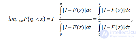 (2.47)
because
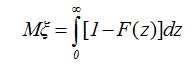 (2.48)
(for more detail see mathematical appendix 4).
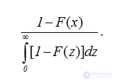
Consequently, the density of the limiting distribution equals
.
For the forward recurrence time we need to pass to the limit in relation (2.41), using the key renewal theorem. The upper limit of the definite integral in (2.41) equals t, so under the integral sign stands the function Q(t-y)=1-F(t+x-y). Consequently, we have Q(t)=1-F(t+x).
The limit of the first term equals unity and we finally obtain
. 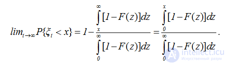 (2.49)
Thus the coincidence of the limiting distributions for the forward and backward recurrence times is proved.
To determine the limiting joint distribution we need to pass to the limit in equality (2.44). In this case Q(t)=1-F(t+x+y) and therefore
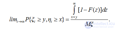 (2.50)
Let us note the dependence of the random variables ξt and ηt in the limiting case as well. The last statement follows from equality (2.50).
Now for the limiting case let us determine the expectation of the interval covering an infinitely distant point t. The length of this interval equals ξt+ηt. If we use equality (2.48) for the expectation of a positive random variable and the limiting equalities (2.42) and (2.44), then we can assert that the expectation of this interval equals
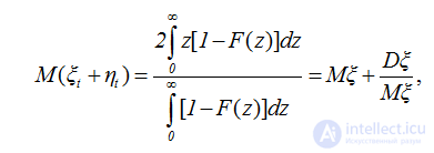 (2.51)
where Dξ denotes the variance of the random variable, if it exists. As follows from equality (2.51), the expectation of the interval under study does not coincide with the expectation Mξ and differs the more, the greater the variance of the random variable ξ. In deriving equality (2.51) we used the property of the expectation of a sum of even dependent terms. The same result is obtained if we pass directly to the limit in equality (2.39).
To determine this limiting distribution we need to pass to the limit in equality (2.45). Equality (2.45) can be transformed by the change of the integration variable z=t-ν
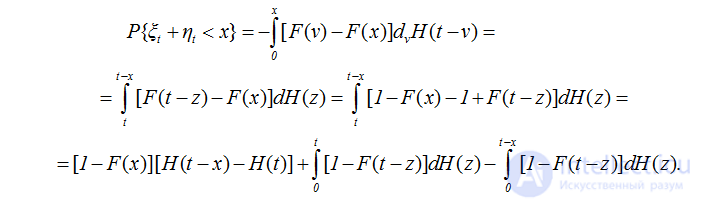
The first term has a limit equal to 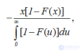 on the basis of Blackwell's theorem, the second term has unity as its limit, since the equality
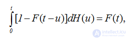 if we use the integral renewal equation (2.16) or the key renewal theorem, finally, the last term has as its limit if we use the key renewal theorem.
Finally we obtain
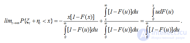 (2.52)
From equality (2.18), by elementary transformations, we obtain
.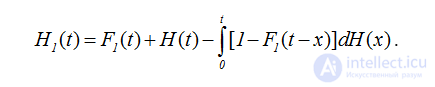
For the function H(t) we use the asymptotic expansion (2.22), and for the last integral, on the basis of the key renewal theorem, we have
.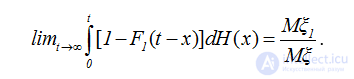
Therefore for the renewal function of a delayed renewal process we obtain
. 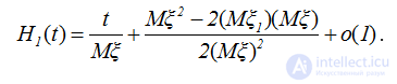 (2.53)
In conclusion of this section we once again note that the formulas obtained for the limiting distributions are valid for a non-arithmetic (non-lattice) distribution F(x).

Comments