
Lecture
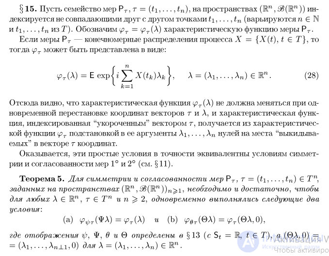
Let a family of measures PT, T = (?]_,..., ?n), on the spaces (En, S^iW1)) be indexed by pairwise distinct points t\,..., tn (with n E N
and t1,..., tn from T). Denote by ipT = (pT(\) the characteristic function of the measure PT.
If the measures PT — are the finite-dimensional distributions of the process X = {X(?), t G T}, then
ipT can be represented in the form:
>T(A) = E exp(i ^ X
A = (A1, ..., An) e Rn. B8)
From this it is clear that the characteristic function It turns out that these simple conditions are exactly equivalent to the symmetry and consistency conditions 1° and 2° (see § 11).
Theorem 5. For the symmetry and consistency of the measures PT; T = (t1,..., tn) G Tn, defined on the spaces (En, ^(En))n^i, it is necessary and sufficient that
for all A G ln, T G Tn and n ^ 2, the following two conditions hold simultaneously:
(a) ^
where the maps p, P, t and O are defined in § 13 (with St = E, t G T), and (OA, 0) =
= (A1,..., An_Li, 0) for A = (A1,..., An) G E™.
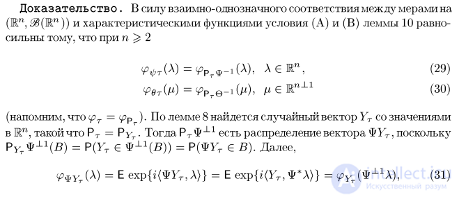
Proof. By virtue of the one-to-one correspondence between measures on
(En, S^iW1)) and characteristic functions, conditions (A) and (B) of Lemma 10 are equivalent to the fact that for n ^ 2
^rW=VPr*-i(A), AGE", B9)
?>eTM=?>Pre-iM, ^K1 C0)
(recall that <pT = <^p ) • By Lemma 8 there exists a random vector YT with values
in Em, such that PT = PYT. Then PT-P-1-1 is the distribution of the vector PYT, since
€ B). Further,
?»PYT(A) = E exp{i(PYT,L)} = E exp{i(YT,P*A)} = ^(YT,PA), C1)
where we identify P with the orthogonal matrix defining this map (so that P* = p-11, P* — is the transpose of P). By C1) condition B9)
takes the form (p^T(\) = (^T(p-11L), L E En, which is equivalent to condition (a).
Similarly,
E exp{i@FT,/i)} =
E exp{i(FT, (
C2)
Thus, C0) is equivalent to condition (b). D
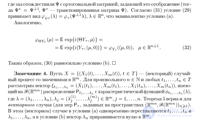
Remark 4. Let X = {(X1(t),... ,Xm(t)), t G T} — be a (vector-valued) random process with values in Em. For an arbitrary n E N and any t1,..., tn G T
consider the vector 6t1,...,tn = (X1(t1), • • • ,Xm(t1),... ,X1(?n),... ,Xm(tn)), having on B (Emn) the distribution Pt1,... ,tn with characteristic function 0t1,... ,tn (A),
= (A^
^m)
where L = (A1,... ,An), Aj = (A^,... ,A^-m)) G Em, j = l,...,n. Theorem 5 also holds for the
vector case (for measures PT, defined on the spaces (Em
In this (vector) case, in condition (a) t1,..., tn and
A1,..., An are permuted simultaneously, and in condition (b) the vector An is set equal to zero in Em.
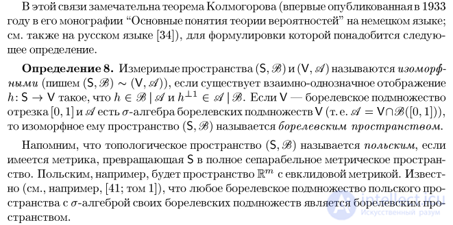
Kolmogorov's theorem (first published in 1933 in his monograph "Grundbegriffe der Wahrscheinlichkeitsrechnung" [Foundations of the Theory of Probability] in German;
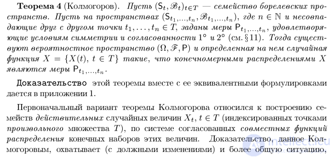
see also in Russian [34]) is remarkable, and to state it we shall need the following definition.
Definition 8. Measurable spaces (S, S&) and (V, si) are called isomorphic (written (S, S§) ~ (V, si)) if there exists a one-to-one map
h: S —У V such that h G B \ sd and H±g G sd \ B&. If V — is a Borel subset of the segment [0,1] and sd is the sigma-algebra of Borel subsets of V (i.e. «c/ = Vn5S([0,1])), then the space (S, J) isomorphic to it is called a Borel space.
Recall that a topological space (S, S§) is called Polish if there is a metric turning S into a complete separable metric space. For example, the space Em with the Euclidean metric is Polish. It is known (see, e.g., [41; vol. 1]) that any Borel subset of a Polish space, with the sigma-algebra of its own Borel subsets, is a Borel space.
Theorem 4 (Kolmogorov). Let (St,8$t)teT — be a family of Borel spaces. Suppose that on the spaces (St1,...,tnJ^t1,...,tn)J, where n G N and the pairwise distinct points t1,..., tn G T, measures Pt1,...,tn are given, satisfying the symmetry and consistency conditions 1° and 2° (see § 11). Then there exist a probability space (Omega, F, P) and a random function X = {X(t), t G T} defined on it such that the finite-dimensional distributions of X
are the measures Pt1,...,tn-
The proof of this theorem, together with its equivalent formulations, is given in Appendix 1.
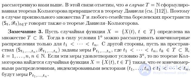
The original version of Kolmogorov's theorem concerned the construction of families of real-valued random variables Xt, t G T (indexed by points
of an arbitrary set T), from a system of consistent joint distribution functions of finite collections of these variables. The proof given by Kolmogorov also covers (with due modifications) the more general situation considered above. In this connection we note that in the case T = N the stated Kolmogorov theorem turns into Daniell's theorem (see [112]). Therefore, in the case of an arbitrary set T and any family of Borel spaces (St, S%t)teT, one also speaks of the Daniell–Kolmogorov theorem.
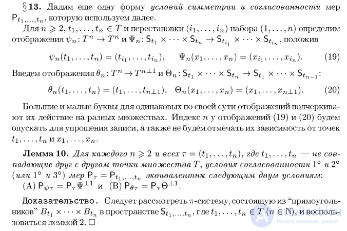
Remark 3. Let a random function X = {X(t), t G T} be defined on a set T C R. Then, by virtue of condition 1°, one may consider finite-dimensional
distributions only for t\ < • • • < tn. On the other hand, suppose that on the spaces (St1,...,tn, ^t1,...,tj measures P*1,...,*„ are given, where h < • • • < tnj tk G T C E,
k = l,...,n,n G N. If these measures satisfy condition 3°, then by Kolmogorov's theorem there exists a random function X = {X(t), t G T} such that its finite-dimensional distributions, indexed by vectors (t1,..., tn) with t\ < • • • < tn,
are the measures Pt1,...,tn.
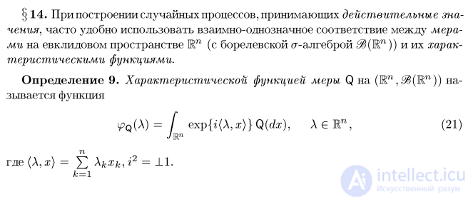
13. Let us give one more form of the symmetry and consistency conditions for the measures
Pt1,... ,tn ? which we shall use later.
For n ^ 2, t1,..., tn G T and a permutation (i1,..., in) of the tuple A,..., n) define
the maps фп: Tn ->• Tn and Фп: S^ x • • • x Stn ->• St • x • • • x S^ , by setting
^nOi,...,?n) = (?^,...,?0, ФпOi,...,жп) = (xi1,...,xin). A9)
Introduce the maps вп: Tn ->• T71-11 and 0П: St: x • • • x Stn ->• St: x • • • х Stn_1:
^n(*i, • • •, tn) = (*i, • • •, tn±1), вп(ж1,..., жп) = (ял,..., xn_Li). B0)
Upper- and lower-case letters, for maps that are identical in substance, emphasize their action on different sets. We shall omit the index n on the maps A9) and B0)
for the sake of brevity, and likewise shall not indicate their dependence on the points
Lemma 10. For every n ^ 2 and all T = (t1,... ,tn), where t1,... ,tn — are pairwise distinct points of the set T, the consistency conditions 1° and 2°
(or 1° and 3°) of the measures PT = Pt1,...,tn are equivalent to the following two conditions:
(А) р^т = ртф±х и (в)'р"вт = р.е^1.
Proof. One should consider the pi-system consisting of "rectangles" Btx x • • • x Btn in the space Stx,... ,tn ? where t1,..., tn G T (n G N), and use Lemma 2. ?
§ 14. In constructing stochastic processes taking real values, it is often convenient to use the one-to-one correspondence between measures on the Euclidean space W1 (with the Borel sigma-algebra S^iW1)) and their characteristic functions.
Definition 9. The characteristic function of a measure Q on (ЕП,^(ЕП)) is the function
=/ exp{i(X,x)}Q(dx), AGEn, B1)
n
where (A, ж) = ? \kxk,i2 = -LI-
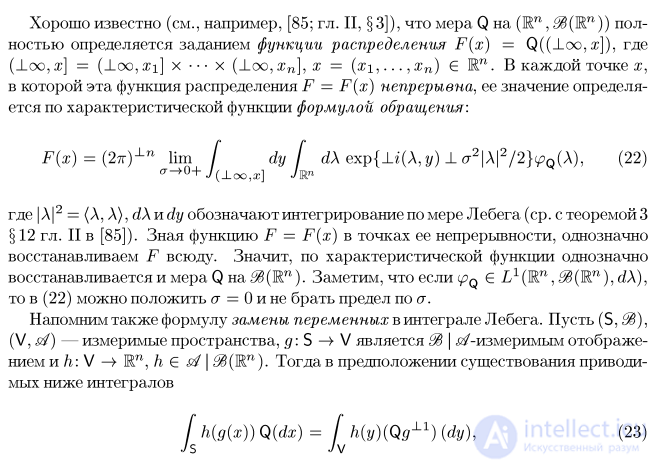
It is well known (see, e.g., [85; ch. II, § 3]) that a measure Q on (Еп, ?ё(Шп)) is completely determined by specifying the distribution function F(x) = Q((_Loo,x]), where
(_Loo, x] = (-Loo, xi] x • • • х (_Loo, xn], x = (x\,..., xn) G En. At every point x,
at which this distribution function F = F(x) is continuous, its value is determined via the characteristic function by the inversion formula:
F(x) = Bтг)±п lim / dy I dX exp{±i(X,y) _L a2|A|2/2}^Q(A), B2)
^°+ J(±oo,x] Jwi
where | A|2 = (A, A), dX and dy denote integration with respect to Lebesgue measure (cf. Theorem 3
§ 12 ch. II in [85]). Knowing the function F = F(x) at its points of continuity, we uniquely
recover F everywhere. Hence the characteristic function also uniquely
determines the measure Q on ?$(ЕП). Note that if (^q E L1 (Еп, ?$(ЕП), dX),
then in B2) one may set a — 0 and not take the limit over a.
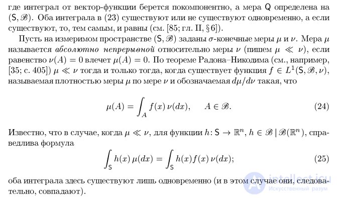
Let us also recall the change-of-variables formula for the Lebesgue integral. Let (S, Зё),
(V, si) — be measurable spaces, g: S —> V being a Зё \ ^/-measurable map, and h: V —у En, h € si \ ^(En). Then, assuming existence of
the integrals below,
/ h(g(x)) Q(dx) = / h(y)(Qg±1) (dy), B3)
is Jv
where the integral of a vector-valued function is taken componentwise, and the measure Q is defined on (S, SS). Both integrals in B3) exist or fail to exist simultaneously, and if they
exist, then, accordingly, they are equal (see [85; ch. II, § 6]).
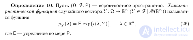
Let sigma-finite measures /i and is be given on a measurable space (S,3e). The measure \i is called absolutely continuous with respect to the measure is (written \± <$С is), if
the equality is (А) = 0 implies fi(A) = 0. By the Radon–Nikodym theorem (see, e.g., [35; p. 405]) \± ^С v if and only if there exists a function / G I/1(S, Й§, is),
called the density of the measure \i with respect to the measure v and denoted dfi/dis, such that = / f(x)u(dx), A€<%. B4)
J А
It is known that when \i ^C is, for a function h: S —> En, h G Зё \ ?$(ЕП), the formula
/ h(x) fi(dx) = / h(x)f(x) u(dx); B5)
holds; both integrals here exist only simultaneously (and in that case they are, consequently, equal).
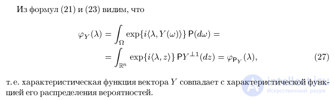
Definition 10. Let (Omega, &, P) — be a probability space. The characteristic function of a random vector Y: Omega —у En (Y G 3* \ SftiW1)) is called-
the function ipY(X) = Е exp{i(A,F)}, A G Еп, B6)
where Е — denotes averaging with respect to the measure P.
From formulas B1) and B3) we see that
= [ exp{i(\,z)}PY±1(dz)=(PpY(\), B7)
i.e. the characteristic function of the vector Y coincides with the characteristic function of its probability distribution.
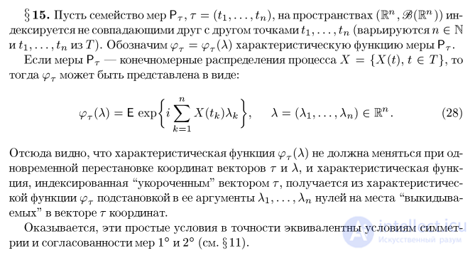
§ 15. Let a family of measures PT, T = (?]_,..., ?n), on the spaces (En, S^iW1)) be indexed by pairwise distinct points t\,..., tn (with n E N
and t1,..., tn from T). Denote by ipT = (pT(\) the characteristic function of the measure PT.
If the measures PT — are the finite-dimensional distributions of the process X = {X(?), t G T}, then
ipT can be represented in the form:
>T(A) = E exp(i ^ X
A = (A1, ..., An) e Rn. B8)
From this it is clear that the characteristic function function, indexed by the "shortened" vector T, is obtained from the characteristic function ipT by substituting zeros into its arguments A1,..., An at the places of the "discard-
ed" coordinates in the vector T.
It turns out that these simple conditions are exactly equivalent to the symmetry and consistency conditions 1° and 2° (see § 11).
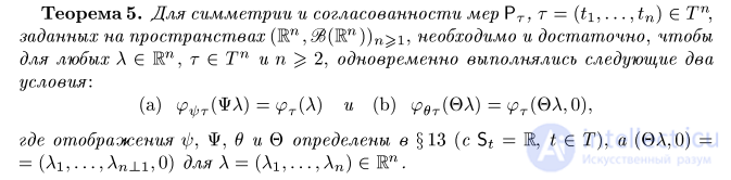
Theorem 5. For the symmetry and consistency of the measures PT; T = (t1,..., tn) G Tn, defined on the spaces (En, ^(En))n^i, it is necessary and sufficient that
for all A G ln, r G Tn and n ^ 2, the following two conditions hold simultaneously:
(a) ^
where the maps p, P, в and O are defined in § 13 (with St = E, t G T), and (OA, 0) =
= (A1,..., An_Li, 0) for A = (A1,..., An) G E™.
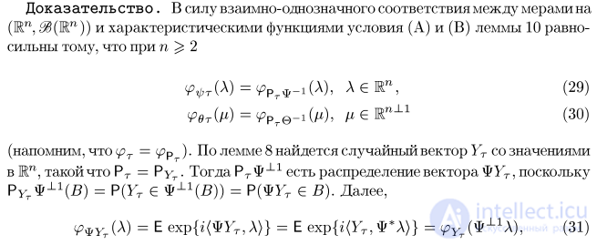
Proof. By virtue of the one-to-one correspondence between measures on (En, S^iW1)) and characteristic functions, conditions (A) and (B) of Lemma 10 are equivalent to the fact that for n ^ 2 ^rW=VPr*-i(A), AGE", B9) ?>eTM=?>Pre-iM, ^K1 C0) (recall that <pT = <^p ) • By Lemma 8 there exists a random vector YT with values in Ж™, such that PT = PYT. Then PT-Ф-1-1 is the distribution of the vector ФYT, since
€ Б). Further,
?»ФYT(A) = Е ехр{г(ФYT,Л)} = Е ехр{г(YT,Ф*А)} = ^(YT,Ф*А), C1)
where we identify Ф with the orthogonal matrix defining this map (so that Ф* = ф-11, Ф* — is the transpose of Ф). By C1) condition B9)
takes the form (p^T(\) = (^T(ф-11Л), Л Е Еп, which is equivalent to condition (a).
Similarly,
Е exp{i@FT,/i)} =
Е exp{i(FT, (
C2)
Thus, C0) is equivalent to condition (b). D
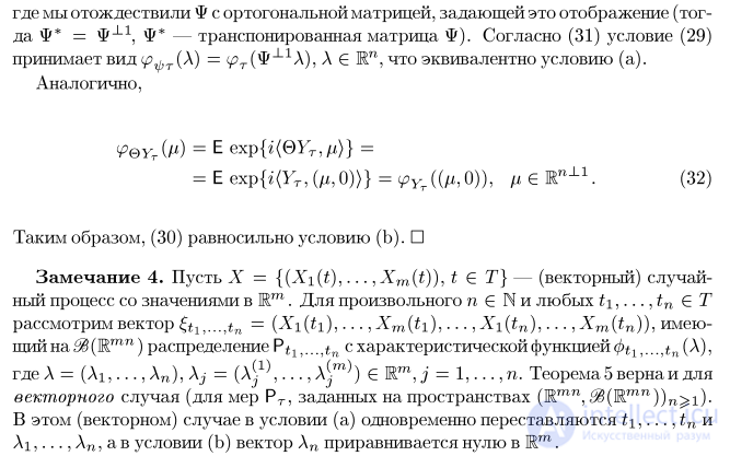
Remark 4. Let X = {(X1(t),... ,Xm(t)), t G T} — (vector-valued) random process with values in Em. For an arbitrary n E N and any t\,..., tn G T
consider the vector 6b...,tn = (X1(t1), • • • ,Xm(t1),... ,X1(?n),... ,Xm(tn)), having on Зё (Emn) the distribution Ptx,... ,tn with characteristic function 0t1,... ,tn (A),
= (A^ ^m) where L = (A1,... ,An), Aj = (A^,... ,A^-m)) G Em, j = l,...,n.
Theorem 5 also holds for the vector case (for measures PT, defined on the spaces (Em In this (vector) case, in condition (a) t1,..., tn and A1,..., An are permuted simultaneously, and in condition (b) the vector An is set equal to zero in Em.

Comments