
Lecture
Hohmann transfer orbit in celestial mechanics — an elliptical orbit used to transfer between two other orbits, usually located in the same plane. In the simplest case it intersects these two orbits at apoapsis and periapsis . The orbital maneuver for the transfer includes two engine burn impulses — one for entering the Hohmann trajectory and one for leaving it. It is named after the German scientist Walter Hohmann, who described it in his book in 1925. Hohmann was greatly influenced by the science fiction writer Kurd Lasswitz's 1897 book «On Two Planets». The same trajectory was independently proposed by the Soviet scientists Vladimir Vetchinkin and Friedrich Zander.
The Hohmann trajectory is theoretically calculated for two impulsive (conditionally instantaneous) velocity increments. However, since the engine burn time needed to achieve the corresponding velocity increment differs from zero, and the impulse should be as short as possible, engines with high thrust are required. If the spacecraft is equipped only with low-thrust engines, then performing the transfer along a Hohmann trajectory will require several engine firings, which sharply reduces the energy advantage of the transfer along such a trajectory (the required velocity increment amounts to up to 141% of the two-impulse maneuver).
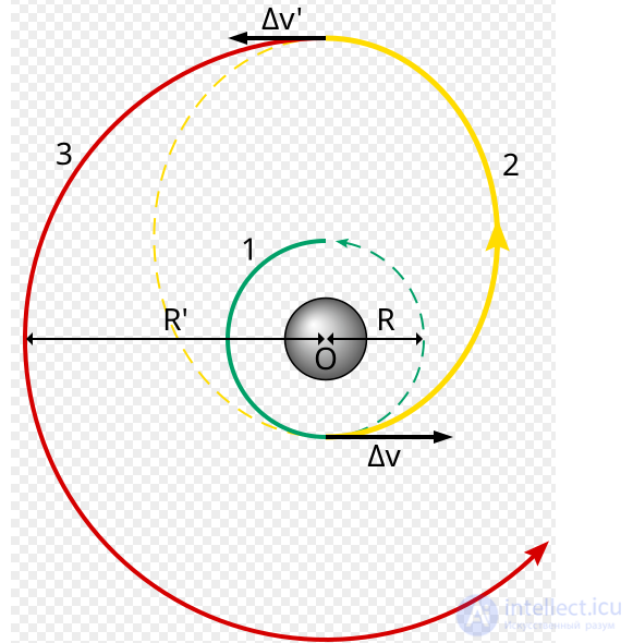
Hohmann transfer trajectory (yellow) from a low circular orbit (green) to a higher circular orbit (red). Δv and Δv' — the first and second engine burns for acceleration.
For a Hohmann trajectory, the angular range (the angle between the rays drawn from point O to the initial and final points of the trajectory) equals 180°. If it is less than 180°, the trajectory is called a first-half-revolution trajectory, or type 1, and if it is greater — a second-half-revolution trajectory, or type 2.
Hohmann orbits are the most fuel-economical two-impulse maneuvers, but they do not provide the minimum transfer time . A shorter time is possible when performing an energy-costly hyperbolic transfer.
For certain ratios of parameters between the initial and final orbits (when the semi-major axes differ by a factor of 12 or more), there exists a slightly more fuel-economical (by fractions of a percent of the Δv budget) three-impulse orbital maneuver, in which two elliptical transfer orbits are used sequentially. However, this maneuver is significantly longer and requires two orders of magnitude more time than the Hohmann trajectory to achieve significant savings (for example, several thousand years for flights from Earth to the outer planets, compared to tens of years for the Hohmann orbit).
The calculation of the necessary velocity increments can be performed in two ways: by setting the ratio of the radii of the final and initial orbits, or by setting the orbital velocities of the initial and final orbits. The second way is simpler if the orbital velocities of the orbits are already known.
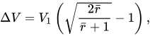
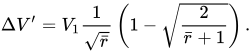
If the ratio of the orbital radii  and the orbital velocity of the initial orbit
  are known, then the velocity increments are equal to
If the orbital velocities of the initial V1 and final V2 orbits are known, then the velocity increments are calculated as follows:
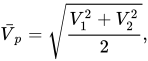
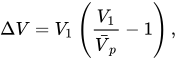
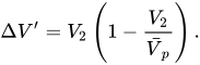
The given relations are valid only for circular initial and final orbits and hold both when transferring from a low orbit to a high one and when transferring from a high orbit to a low one. In the second case the increments turn out to be negative, which means that the spacecraft needs to be decelerated by the resulting amount.
The total increment needed to transfer from one orbit to another can be represented as

where the function  represents the coefficient of the total increment, which depends on the ratio of the orbital radii. Analysis of it shows the following interesting things. First, the total increment is always less than the difference between the orbital velocities of the final and initial orbits. Moreover, the difference in these quantities increases with the growth of the coefficient
  . Second, this function has a maximum at r¯≈15.582
 . The value of the function at this point equals
  . This means that the most energy-costly transfer will be a transfer from a low orbit to a high orbit whose altitude is 15.582 times greater than the low orbit. A transfer to an even higher orbit (as well as to a lower one) will be less costly. As tends to infinity, that is, when reaching the second cosmic velocity at this point, the value of the function equals
  . This is because the first impulse ΔV, although it increases monotonically to the value
  as the altitude of the final orbit increases, but from a certain point the required level of the second impulse
  begins to fall to zero, which in turn is related to the decrease to zero of the orbital velocity of the final orbit. When transitioning from a high orbit to a low one, this effect is not observed. In this case the function decreases monotonically to infinity. However, if we take two given orbits, the total velocity increments are equal both when accelerating and transitioning from a low orbit to a high one, and when decelerating and transitioning from a high orbit to a low one.
When using the Oberth effect to move a spacecraft from the orbit of one planet to the orbit of another, it allows the use of a smaller delta-v than the sum of the delta-v values for separate maneuvers to leave the first planet, then perform a Hohmann transfer to the second planet, and then enter orbit around the other planet.
For example, consider a spacecraft flying from Earth to Mars. At the start of its journey the spacecraft will already have a certain velocity and kinetic energy associated with its orbit around Earth. While the rocket engine operates it applies its delta-v, but the kinetic energy increases quadratically until it becomes sufficient to escape the planet's gravitational potential, and then it burns more to obtain enough energy to enter a Hohmann transfer orbit (around the Sun). Because the rocket engine is able to make use of the initial kinetic energy of the propellant, much less delta-v is required beyond what is needed to reach escape velocity, and the optimal situation is one in which the transfer impulse is produced at the minimum altitude (small periapsis) above the planet. The required delta-v is only 3.6 km/s, which is only about 0.4 km/s more than what is needed to leave Earth, although this results in the spacecraft moving 2.9 km/s faster than Earth, heading toward Mars (see table below).
At the other end of the trajectory, the spacecraft must slow down so that Mars's gravity can capture it. This capture impulse is optimally performed at low altitude, in order to make maximum use of the Oberth effect. Consequently, organizing the transfer requires relatively little thrust at both ends of the trajectory compared to the situation in open space.
However, in any Hohmann transfer, the alignment of the two planets in their orbits is crucial: the destination planet and the spacecraft must arrive at the same point in their orbits around the Sun at the same time. This alignment requirement gives rise to the concept of launch windows.
For the Moon, the term «lunar transfer orbit» (LTO) is used.
The formula above can be used to calculate Δv (in km/s) required to enter a Hohmann transfer orbit to reach various destinations from Earth (assuming the planets move in circular orbits). In this table, the column «Δv to enter a Hohmann orbit from Earth's orbit» shows the change in Earth's velocity to the velocity required to enter the Hohmann ellipse, the other end of which will be at the desired distance from the Sun. The column «Altitude at LEO» shows the required velocity (in a non-rotating frame centered on Earth) at an altitude of 300 km above Earth's surface. It is obtained by adding to the specific kinetic energy the square of the escape velocity (10.93 km/s) from that altitude. The column «LEO» represents simply the previous velocity minus the orbital velocity at LEO, equal to 7.73 km/s.
| Destination | Orbital radius ( AU ) |
Δ v (km/s) to enter Hohmann orbit from | ||
|---|---|---|---|---|
| Earth's orbit | LEO altitude | LEO | ||
| Sun | 0 | 29.788 | 31.732 | 24.002 |
| Mercury | 0.39 | 7.474 | 13.239 | 5.509 |
| Venus | 0.72 | 2.532 | 11.221 | 3.491 |
| Mars | 1.52 | 2.929 | 11.320 | 3.590 |
| Jupiter | 5.2 | 8.792 | 14.031 | 6.301 |
| Saturn | 9.54 | 10.290 | 15.015 | 7.285 |
| Uranus | 19.19 | 11.282 | 15.714 | 7.984 |
| Neptune | 30.07 | 11.655 | 15.981 | 8.251 |
| Pluto | 39.48 | 11.815 | 16.100 | 8.370 |
| Infinity | ∞ | 12.338 | 16.481 | 8.751 |
Note that in most cases Δ v from low Earth orbit is less than Δ v for entering a Hohmann orbit from Earth's orbit.
To get to the Sun, it is not actually necessary to use Δ v at 24 km/s. One could use 8.8 km/s to travel very far from the Sun, then use a negligibly small Δ v, to reduce the angular momentum to zero, and then fall onto the Sun. This is also known as a bi-elliptic transfer, which is a sequence of two Hohmann transfers. In addition, the table does not list the values that would apply when using the Moon for a gravity assist. There are also possibilities for using a single planet, such as Venus, which is the easiest to reach, to help achieve other planets or the Sun.
A bi-elliptic transfer consists of two semi-elliptical orbits. On the initial orbit, the first engine impulse increases the delta-v to move the spacecraft into the first transfer orbit with an apocenter at some point.rb from the central body. At this point, the second engine impulse moves the spacecraft into the second elliptical orbit with a pericenter coinciding with the radius of the final desired orbit, where a third impulse is made, placing the spacecraft into the desired orbit. [ 11 ]
Although some bi-elliptic transfers require one more engine burn than a Hohmann transfer, and generally require more travel time, some bi-elliptic transfers require a smaller total delta-v than a Hohmann transfer when the ratio of the final to initial semi-major axis is 11.94 or greater, depending on the intermediate semi-major axis chosen. [
The idea of the bi-elliptic transfer trajectory was first published by Ary Sternfeld in 1934. [ 13 ]
Low-thrust engines can approximate a Hohmann transfer orbit by gradually expanding the initial circular orbit through carefully timed engine burns. This requires a change in velocity (delta- v ) greater than that of a two-impulse transfer orbit [ 14 ] , and takes more time.
Engines such as ion engines are more difficult to analyze using the delta- v model. These engines provide very low thrust while offering a significantly higher delta- v budget, significantly higher specific impulse, and less propellant and engine mass. A two-burn Hohmann maneuver would be impractical at such low thrust; this maneuver mainly optimizes propellant use, but in this situation there is relatively plenty of it.
If only low-thrust maneuvers are planned during a mission, then continuous operation of a low-thrust but very high-efficiency engine can provide a large delta- v while using less propellant than a conventional chemical rocket engine.
Transferring from one circular orbit to another by gradually changing the radius simply requires the same delta- v, as the difference between the two velocities. [ 14 ] Such a maneuver requires a greater delta- v, than the two-speed Hohmann maneuver, but it is performed with constant low thrust rather than a brief application of high thrust.
The amount of propellant used measures the efficiency of the maneuver and the equipment used for it. The total delta- V used measures only the efficiency of the maneuver. In electric propulsion systems, which generally have low thrust, the high efficiency of the propulsion system usually compensates for the higher delta-V compared to the more efficient Hohmann maneuver.
Transfer orbits using electric propulsion or low-thrust engines optimize the transfer time to reach the final orbit, rather than delta-v, as in a Hohmann transfer orbit. For a geostationary orbit, the initial orbit is set to be supersynchronous, and by continuously increasing thrust in the direction of velocity at apogee, the transfer orbit is converted into a circular geosynchronous orbit. However, this method requires much more time due to the low thrust applied to the orbit.
In 1997, a set of orbits known as the Interplanetary Transport Network (ITN) was published, offering even lower delta- v (although much slower and longer) paths between various orbits than Hohmann orbits. [ 16 ] The Interplanetary Transport Network differs in nature from Hohmann transfers, since Hohmann transfers assume the presence of only one large body, whereas the Interplanetary Transport Network — does not. The Interplanetary Transport Network is able to use a lower delta- v by taking advantage of gravity assists from planets.

Comments