2.3 Elementary links

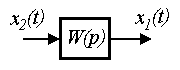
Elementary links are called the simplest components (blocks) of a system whose behavior is described by algebraic equations or differential equations of the 1st – 2nd order:

(2.50) ,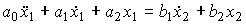

Where - output variable - input variable - constant coefficients (parameters). Equation (2.50) can be written in operator form:

,

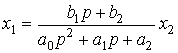those. the transfer function of the link is

(2.51) .

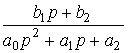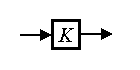
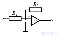
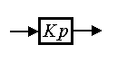
Proportional (inertia-free) link . The link is described by an algebraic equation.

(2.52) ,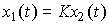

Where - coefficient of proportionality, which (due to the lack of inertial properties of the block) coincides with the static characteristic. Proportional transition function -

(2.53) .

Examples: measuring potentiometers, gearboxes, voltage amplifiers ( ) etc.

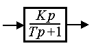
Aperiodic link. The link is described by a differential equation

(2.54)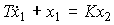

or, in reduced form, by the equation

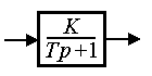
(2.55) ,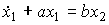

Where - coefficient, - time constant, a = K / T, b = 1 / K. The operator form of the link has the form

(2.56)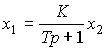

or accordingly

(2.57) ,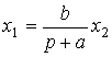

The transition function of the link is determined by the expression

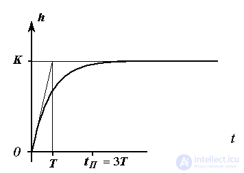
Fig. 2.10. Transition function aperiodic link

(2.58) ,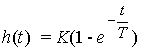

and the static characteristic is

(2.59) .

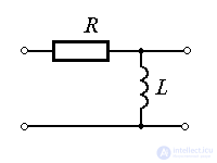
Examples: power amplifiers, thermal processes, engine acceleration process - chain (see example 1.1), LR chain.

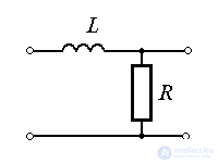
Integrating link. The link is described by a differential equation

(2.60)

or, in operator form

(2.61) .

Transition function integrator

(2.62) .

The link belongs to astatic blocks and therefore has no static characteristic.

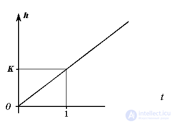
Fig. 2.11. Transition function integrator

Examples: elements of mechanical systems (see the movement of a material point, example 2.3), described by the equations of the dynamics of a type

,

and kinematic equations

;

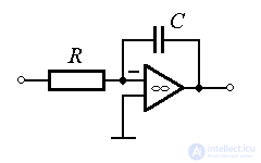
electronic integrators ( ) etc.

Differentiating link (perfect). The link is described by a differential equation

(2.63)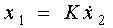

or, in operator form,

(2.64) .

Differential Link Transition Function -

(2.65) ,

and the response of the link to the linearly increasing signal x ₂ = t -

(2.66) .

When x ₂ = const for any t> 0 , and, therefore, the static characteristic of the link is a direct .

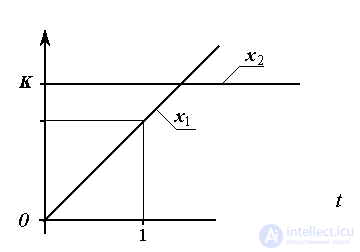
Fig. 2.12. Differentiator response on linearly increasing impact

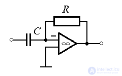
Examples: tachogenerator (electric speed sensor), electronic differentiator ( ).

Remark 2.4 . The output of the differentiating link is the derivative of the input signal, i.e. its instant speed is dx ₂ / dt . The operation of finding the current value of the velocity x ₁ (t) = dx ₂ (t) / dt only from the information about the signal at the given time t currently x ₂ (t) is not physically realizable and therefore there are no ideal differentiating links. However, the derivative can be approximated as ₁ (t) = D x ₂ (t) / D t , where D t is the time interval, D x ₂ is the corresponding signal increment x ₂ . By reducing the interval D t you can get the value ₁ (t) , arbitrarily close to the current speed value x ₁ (t) . Consequently, despite the unrealizability (with absolute precision) of the operation of differentiation, it is theoretically possible to build a link that ensures finding the derivative dx ₂ (t) / dt with arbitrarily high accuracy.

Real differentiating link. The link is described by the equation

(2.67) .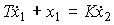

or, in operator form,

(2.68)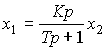

The transition function of the link is

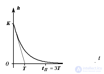
Fig. 2.13. Transition function of a real differentiator

(2.69) ,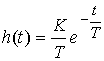

and the response of the link to the linearly increasing signal x ₁ = t coincides with the transition function of the aperiodic link, i.e.

(2.70) .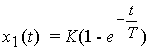

When x ₂ = const and performed that corresponds to the static characteristic of the link.

With sufficiently small time constants T , the characteristics of the link approach the characteristics of the ideal differentiating link (see Remark 2.4).

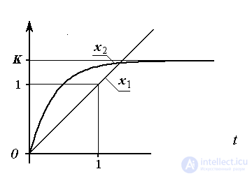
Fig. 2.14. Real Differential Link Reaction on linearly increasing impact

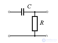
Examples: CR and RL chains.

Oscillating link . The link is described by a 2nd order differential equation.

(2.71) ,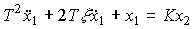

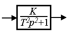
- time constant - attenuation parameter, or operator equation (2.50), where the transfer function is

(2.72) .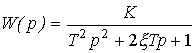

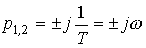
The roots of the characteristic equation take values

,

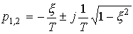
Where - attenuation coefficient, 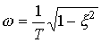- The angular frequency of oscillation.

The transition function of the link is

(2.73) ,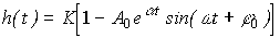

Where 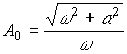; 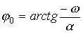, and the static characteristic is

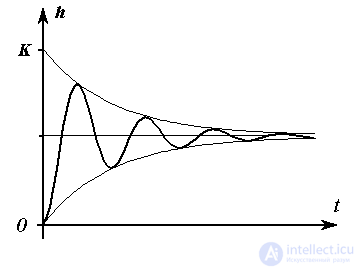
Fig. 2.15. Oscillating transition function

(2.74) .

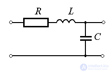
Examples: pendulum in a viscous medium, - chain.

Remark 2.5. In the limiting case, At the output of the link, continuous oscillations occur, and - monotonous (aperiodic) process, which corresponds to the conservative and double aperiodic link considered below.

Conservative link (oscillator). The link is described by a differential equation

(2.75)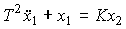

or operator equation (2.50), where

(2.76) ,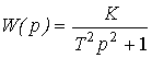

and is obtained from the oscillatory level when . Conservative link has pure imaginary poles.

and transition function

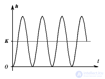
Fig. 2.16. Oscillating transition function

(2.77) ,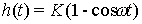

Where . The link has no static characteristic.

Examples: pendulum in vacuum; ideal oscillatory (LC) circuit.

Double aperiodic link. The link is described by the equation

(2.78)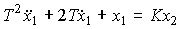

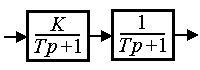
or operator equation (2.50), where

(2.79) .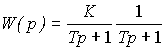

The link has equal real roots of the characteristic equation

,

and transient function

(2.80) .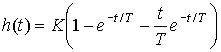

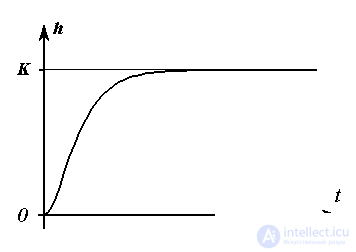
Fig. 2.17. Double aperiodic transition function

Static Link Characterization

(2.81) .