Algorithmic complexity (Big O) in SQL SELECT queries and with JOINs

Practice

In the world of software development, the efficiency of database query execution plays a key role in ensuring application performance. In this context, understanding algorithmic complexity (Big O notation) when retrieving data from a database using SQL becomes an important aspect for developers and system architects. Algorithmic complexity in SQL depends on various factors, such as the presence of indexes, the structure of the query, the volume of data, and other aspects that affect performance. In this article, we will look at the key aspects of algorithmic complexity when retrieving data in SQL, and how query optimization can significantly affect database performance and, consequently, application behavior.

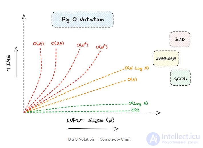
In the context of SQL and data retrieval from a database, evaluating algorithmic complexity using Big O notation is a key point for optimizing query performance. Big O notation provides an abstract representation of how the growth in data volume affects the performance of an algorithm. Let's look at some features of this notation in the context of SQL queries.

O(1) - Constant complexity:
- This case means that the query execution time remains constant regardless of the data volume. For example, a lookup by primary key or index.
O(log N) - Logarithmic complexity:
- Using indexes can reduce query complexity to logarithmic, meaning that execution time grows logarithmically with the data volume. This is often the case when using binary search.
O(N) - Linear complexity:
- Linear complexity means that the query execution time depends linearly on the data volume. An example is a search without using an index.
O(N log N) - Linearithmic complexity:
- This case occurs when query execution combines both linear and logarithmic characteristics. Sorting using indexes can be an example.
O(N^2) and higher - Quadratic complexity and above:
- Such cases can occur when performing complex JOINs or sorting without using indexes.

For queries with multiple joins, the algorithmic complexity (Big O notation) depends on the specific structure of the query, the presence of indexes, and the data volume. Let's look at several cases:

Sequential joins (Nested Loop Join):
- If a query contains sequential joins (for example, INNER JOIN, LEFT JOIN), their complexity can be O(N^2), where N is the number of rows in the tables. This happens because for each row from one table, a search for matching rows in the other table is performed.
Hash-based joins (Hash Join):
- Using hash joins can reduce complexity to O(N), but this depends on the specific implementation and data.
Sorting before joining (Sort-Merge Join):
- If sorting is required before performing the join, the complexity can be O(N log N), where N is the number of rows in the tables.
Using indexes in JOIN:
- If the join is performed using indexes, this can significantly improve performance, reducing complexity to O(log N) or O(N log N), depending on the specific situation.
Multiple JOIN ... JOIN operations:
- In the case of multiple joins, the algorithmic complexity is usually expressed as the product of the complexities of each join. For example, if you have three tables and all of them are joined, the overall complexity could be O(N^3) in the case of sequential joins; for 10 joins without using an index, the complexity would be a gigantic O(N10).

It is important to note that query performance largely depends on the correct use of indexes, the availability of statistics, the query optimizer, and the overall database structure. Performance can vary greatly across different DBMSs and scenarios.

Query optimization includes using indexes, proper database design, writing efficient queries, and using caching. Understanding algorithmic complexity in the context of SQL helps developers make informed decisions to ensure high database performance within their applications.

Closely related to linear execution time is the execution time of plans involving table joins. Here are a few examples:

A hash join has an expected complexity of O(M+N). The classic hash join algorithm for an inner join of two tables first prepares a hash table of the smaller table. The hash table entries consist of the join attribute and its row. The hash table is accessed by applying a hash function to the join attribute. Once the hash table is built, the larger table is scanned, and matching rows from the smaller table are found by looking them up in the hash table.
Merge joins typically have a complexity of O(M+N), but this will strongly depend on the indexes of the join columns and, in the absence of an index, on whether the rows are sorted according to the keys used in the join:
- If both tables are sorted according to the keys used in the join, the query will have a time complexity of O(M+N).
- If both tables have an index on the joined columns, the index already keeps these columns ordered and no sorting is required. The complexity will be O(M+N).
- If neither table has an index on the joined columns, both tables must first be sorted, so the complexity will look like O(M log M + N log N).
- If only one of the tables has an index on the joined columns, then only the table without an index needs to be sorted before the join stage occurs, so the complexity will look like O(M + N log N).
For nested joins, the complexity is usually O(MN). This join is efficient when one or both tables are extremely small (for example, fewer than 10 records), which is a very common situation when evaluating queries, since some subqueries are written to return only a single row.

Algorithmic complexity (Big O) in SQL SELECT queries and with JOINs

Algorithmic complexity O when selecting with sql select * from without using an index

If a SELECT * FROM table query is executed without using an index, the algorithmic complexity can be estimated as O(N), where N is the number of records in the table.

In this case, the database must scan all rows of the table to satisfy the SELECT * FROM table query. This means that the query execution time will be proportional to the number of records in the table.

Using indexes can significantly speed up the data retrieval process, since indexes provide a structured way to search for specific values. However, if indexes are not used, the database is forced to scan all rows, which can be resource-intensive for large tables.

if the id index is used, what is the algorithmic complexity O when selecting with sql select * from where id=N

If you execute a query of the form SELECT * FROM table WHERE id=N and the table has an index on the id column, the algorithmic complexity will be O(log N), where N is the number of records in the table.

Using an index on the id column allows the database to efficiently find the desired record by applying binary search. As a result, executing such a query performs a fast and efficient index lookup, which gives logarithmic complexity.

It is important to note that O(log N) is possible when using balanced data structures for indexes, such as B-trees or B+trees, which provide efficient search over sorted data.

algorithmic complexity O when selecting with a single join in sql select * from table1 join left table2 ON table1 .f=table2.f without and with using an index

If a query of the form SELECT * FROM table1 LEFT JOIN table2 ON table1.f = table2.f is executed, and no index is used for the join (ON table1.f = table2.f), the algorithmic complexity will be O(M * N), where M is the number of records in table1, and N is the number of records in table2.

Without using an index for the join, the database must perform a "nested loop" or a "hash build" to combine records from table1 and table2. In this case, each record from table1 is checked against every record from table2, which results in quadratic complexity.

Using an index for the join could significantly speed up the process, reducing complexity to O(M * log N) or O(M + N) depending on the specific type of index and the optimizations applied by the database.

Algorithmic complexity (Big O) in SQL SELECT queries and with JOINs

Algorithmic complexity O when selecting with sql select * from without using an index

if the id index is used, what is the algorithmic complexity O when selecting with sql select * from where id=N

algorithmic complexity O when selecting with a single join in sql select * from table1 join left table2 ON table1 .f=table2.f without and with using an index

See also

See also

Comments

To leave a comment

Lectures and tutorial on "Databases, knowledge and data warehousing. Big data, DBMS and SQL and noSQL"

Terms: Databases, knowledge and data warehousing. Big data, DBMS and SQL and noSQL