
Lecture
The core of any data warehouse is its data model. Without a data model, it will be very difficult to organize the data in the DW. Therefore, DW developers must spend time and effort developing such a model. Developing the DW model falls on the shoulders of the DW designer.
Compared with designing OLTP systems, the methodology for designing a DW has a number of distinctive features related to orienting the warehouse's data structures toward solving analytical tasks and providing information support for decision-making. The DW data model must ensure an effective solution to precisely these tasks.
The starting point for designing a DW can be the so-called corporate data model (corporate data model or enterprise data model, EDM), which is created during the design of the organization's OLTP systems. When designing a corporate data model, an attempt is usually made to build, on the basis of business operations, a data structure that gathers and synthesizes all the information needs of the organization.
Thus, the corporate data model contains the information necessary for building the DW model. Therefore, at the first stage, if such a model already exists in the organization, the DW designer can begin designing the DW by solving the problem of transforming the corporate data model into the DW model.
How do we solve the problem of transforming a corporate data model into a DW model? To solve this problem, we need to have this model, i.e., the corporate data model must be built and documented. And we need to understand what from this model and how should be transformed into the DW model.
Let us clarify the concept of a corporate data model from the standpoint of the DW designer. By corporate data model is meant a multi-level, structured description of the organization's subject areas, the data structures of the subject areas, business processes and business procedures, data flows adopted in the organization, state diagrams, "data-process" matrices, and other model representations used in the organization's activities. Thus, in the broad sense of the word, a corporate data model is a collection of models of various levels that characterize (model at some abstract level) the organization's activities, i.e., the content of the corporate model directly depends on which model constructs were included in it for a given organization.
The main elements of a corporate data model are:
Thus, the corporate data model contains entities, attributes, and relationships that represent the organization's information needs. Fig. 16.1 shows the main elements of a corporate data model.
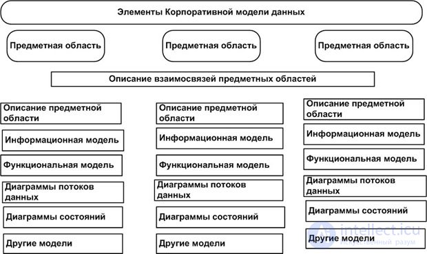
The corporate data model is divided in accordance with subject areas, which represent groups of entities related to supporting specific business needs. Some subject areas may cover such specific business functions as contract management, while others combine entities describing products or services.
Each logical model must correspond to an existing subject area of the corporate data model. If a logical model does not meet this requirement, a model defining the subject area must be added to it.
The corporate data model usually has several levels of representation. At the very highest level (high level) of the corporate data model is a description of the organization's main subject areas and their interrelationships at the entity level. Fig. 16.2 shows a fragment of the top-level corporate data model.
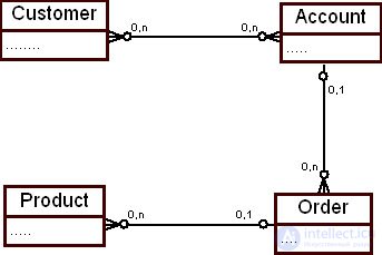
The diagram shown in the figure presents four subject areas: "Customer" ( Customer ), "Account" ( account ), "Order" ( Order ), and "Product" ( Product ). As a rule, at the top level of model representation, only direct relationships between subject areas are indicated, which, for example, capture the following fact: a customer pays an invoice for an order of goods. Detailed information and indirect interrelationships are not shown at this level of the corporate model.
At the next, mid level (mid level) of the corporate data model, detailed information about the objects of the subject areas is shown, i.e., the keys and attributes of entities, their interrelationships, subtypes and supertypes, and so on. For each subject area of the top-level model there is one mid-level model. Fig. 16.3 shows the mid-level representation of the corporate model for a fragment of the "Order" subject area.
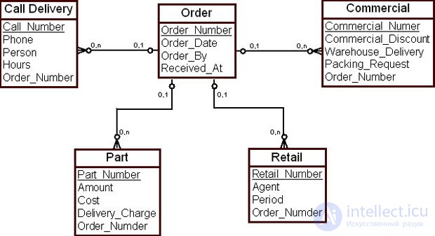
Fig. 16.3 shows that the "Order" subject area ( Order ) includes several entities, defined through their attributes, and the relationships between them. The presented model allows answering such questions as the date of the order, who placed the order, who shipped the order, who receives the order, and a number of others. The diagram shows that this organization distinguishes two types of orders — promotional orders ( Commersial ) and retail orders ( Retail ).
Note that a corporate data model can represent various aspects of an organization's activities, with varying degrees of detail and completeness. If a corporate model represents all aspects of an organization's activities, it is also called an enterprise data model (enterprise data model).
From the standpoint of DW design, an important factor in deciding to create a DW model from a corporate data model is the state of completeness of the corporate data model.
An organization's corporate data model has the property of being evolutionary, i.e., it is constantly developed and improved. Some subject areas of the corporate data model may be well developed, while for others work may not yet have begun. If a fragment of a subject area has not been developed in the corporate data model, then it is not possible to use this model as a starting point for designing the DW.
The degree of completeness of the corporate model can be offset in DW design as follows. Since the process of developing a DW is usually broken down over time into a sequence of stages, its design process can be synchronized with the process of completing the development of individual fragments of the organization's corporate data model.
At the very lowest level of representation of the corporate data model, information is shown about the physical characteristics of database objects corresponding to the logical data model of the mid level of representation of the corporate data model.
Suppose that a corporate data model has been developed in the organization and documented. What actions must the DW designer take to transform it into a DW model?
As a rule, DWs for providing information support to the decision-making process are developed on the basis of a corporate data model. Such DWs form the foundation of decision support systems (DSS). From this standpoint, the main question arises that DW designers for such systems must answer: which data (entity attributes) of the corporate data model should be retained in the DW model, and which can be omitted?
After selecting the data for the DW model, the designer must consider the question of temporal dependencies in the selected data. This is because DWs for DSS usually store time series (historical data) reflecting changes in the model's attribute values over time.
Since the volumes of data stored in a DW are very large, the designer must decide whether to store derived attributes (or computed fields) in the DW. Storing computed values in the DW will increase query processing performance.
After the DW designer has considered the entities and their attributes, they must turn their attention to the relationships between the data and decide which relationships between the data of the corporate data model should be carried over into the DW model.
The next question that the DW designer must resolve has no direct relation to the corporate data model, but must be resolved before the designer begins modeling data according to one of the standard schemas for a DW — "star" or "snowflake". This is the question of the level of data structuring (detail), or data granularity (Data granularity). Recall that the level of data structuring is the degree of detail of the stored data that is optimal from the standpoint of solving information-analytical tasks within the subject area of the DW.
Next, the DW designer can proceed to forming a "star" schema for the DW from the tables of the corporate data model.
Thus, we have the basic algorithm for transforming a corporate data model into a DW model (fig. 16.4):
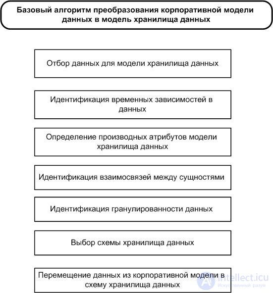
In a modification of this algorithm, according to W.H. Inmon, the DW designer is asked to resolve two additional questions.
The first question concerns identifying periodic groups of data or data arrays and representing them in the DW model (many-to-many relationships).
The second question concerns dividing attributes according to stability parameters, known in the data processing discipline as the "three arrays" question. From the standpoint of processing algorithms, the source data array is split into three arrays: one updated very slowly, one updated periodically, and one updated very quickly.
Let us examine the main steps of the algorithm in more detail.
No unified, formal procedures for selecting attributes of the corporate data model for retention in the DW model have yet been proposed, although research in this direction is being carried out. The main selection criterion is the answer to the question: what is the probability that this attribute will be used in the decision-making process?
The answer to this question can be obtained directly, as a result of a survey or interview of interested parties, namely decision-makers. If the possibility of a comprehensive survey is not available, the DW designer tries to exclude the following data from consideration:
Fig. 16.5 shows an example of selecting data elements of the "Order Item" entity ( Order Item ) of the corporate data model for the DW model.
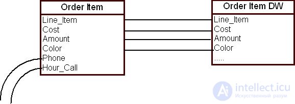
It is unlikely that the attributes "Phone Number" ( Phone ) and "Call Time" ( Hour_call ) will have value for decision-making several months after the order has gone through. Therefore, these attributes can be excluded from the DW model.
The attributes "Order Item" ( line_item ) — in other words, the purchased product, "Cost" ( cost ), and "Quantity" ( amount ) — will almost always be needed for sales analysis. These attributes must be included in the DW model.
It is likely that the "Product Color" attribute ( color ) will be used by the marketing department when planning marketing and advertising activities. For some products, color may not matter from an analysis standpoint. Suppose that the DW designer decided to include this attribute in the DW model.
In the corporate data model of an OLTP system, entities may reflect the current state of the modeled object without tracking the history of changes in these states. From a decision-making standpoint, it may be important how the object of the subject area (represented in the model by this entity) behaves over time, and the DW model must reflect the history of state changes for such an object.
Then, when importing data from the OLTP system into the DW, an instant snapshot of the entity's data will be taken, capturing the state of the object at the moment of import.
The DW designer must introduce into the DW model a timestamp corresponding to the time the snapshot was saved in the DW. Fig. 16.6 shows an example of adding the "Timestamp" attribute ( Time_of_snapshot ) to the DW model for the "Customer" entity ( Customer ) as part of the entity key.
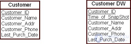
If, in the entities carried over from the corporate data model to the DW model, the temporal attributes are part of a composite entity key, no action by the DW designer is required to change the entity key.
When designing OLTP system databases, derived (computed) data elements are, as a rule, not included in the data structure, and consequently the corporate data model rarely contains such data. Derived data is not included in the corporate data model in order to minimize data redundancy and reduce the number of data elements in the model as much as possible.
The question of whether derived data should be included in the DW model is important from the standpoint of the volume of computation involved in processing data in the DW. If the size of the DW is very large or is growing very fast, it is advisable to include in the data model those data elements which, once computed at DW load time, do not change their values over time.
The designer should bear in mind that including new data elements in the DW model leads to an unnecessary increase in the size of the DW. Therefore, only those derived data elements that are expected to be used fairly often should be included in the DW model.
Thus, the criterion for selecting derived fields for inclusion in the DW model consists of satisfying the following two conditions:
Fig. 16.7 illustrates the procedure for adding derived fields to the DW model using the "Order" entity ( Order ) as an example.
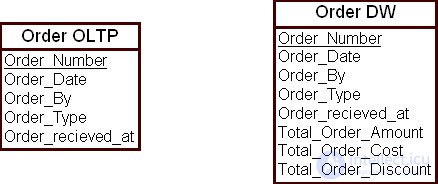
The derived fields of the "Order" entity introduced into the DW model are the attributes "Total Order Quantity" ( total_order_amount ), "Total Order Cost" ( total_order_cost ), "Total Order Discount" ( total_order_discount ). Once an order is closed, these attributes will not change their values. On the other hand, when analyzing the organization's sales within the DW, the probability of these fields being used frequently in queries is high. Therefore, it was reasonable to include these attributes in the DW model.
One of the difficult issues in DW design is the question of transforming the relationships of the corporate data model into DW data relationships. The DW designer must clearly understand the essence of this problem in order to make adequate design decisions that reflect the relationships in the data.
In a corporate data model, as a rule, it is assumed that each relationship between entities captures only a single business rule of the subject area of the OLTP system's database. This relationship between entities is correct at the moment of data access, if the data adequately reflects the state of the entities in the subject area. Such a "point-in-time" character of interpreting a relationship in the corporate data model can lose its meaning when this relationship between data is considered from the standpoint of the historical retrospective characteristic of the DW model.
Let us consider the question of how a relationship between entities of the corporate model can be represented in the DW once data from the OLTP system's database has been loaded into the DW.
As an example, let us examine the relationship between the entities "Parts" ( Part OLTP ) and "Supplier" ( Supplier OLTP ). This relationship reflects the business rule: each product is supplied by a certain supplier. In particular, an organization may adopt the business rule: each product has a primary supplier. Then the integrity constraint is that there are no products in the database that lack a primary supplier. This relationship is valid at the moment of data access (fig. 16.8).
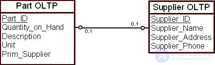
Suppose that data is loaded into the DW on the principle of a periodic point-in-time snapshot. A periodic snapshot of the parts table is taken at the end of a reporting period — end of week, end of month, end of quarter, and so on. Data describing a product is captured in the operational database and placed in the DW at these points in time. This includes the product's primary supplier at the moment the snapshot is taken, i.e., the relationship is represented in the DW through the values of its data at the moment the snapshot was taken.
The "Parts" entity changes its state fairly quickly, since products are constantly being received and shipped from the warehouse. The "Supplier" entity changes its state much more slowly, so a periodic snapshot of the suppliers table is taken, for example, once a quarter. Thus, the supplier recorded in the DW is essentially the most recent supplier of a given product as of the moment the snapshot was taken (fig. 16.9).
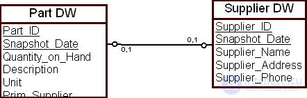
The main drawback of such periodic snapshots is that they may inadequately reflect the state of relationships between entities. Within a week, a product may have five different primary suppliers (i.e., they change each business day), but the snapshot will not reflect such changes. A supplier may ship many different products over a quarter, but the snapshot will show only the last shipment made.
The example shows that, in order to adequately represent the relationship between data in the DW, a historical model of data representation is required for the entities under consideration.
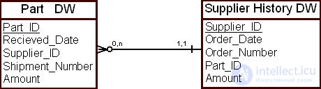
In the historical data model, an entity is treated as a collection of its successive states. For the historical "Parts" table ( Part DW ), when a product is received, all the detailed information is recorded, including the product's supplier. With this approach, the relationship between the two entities, "Parts" ( Part DW ) and "Supplier" ( Supplier DW ), is fully represented in the DW.
If a historical table is also maintained for suppliers, then data about every order for received products placed with a supplier is recorded in it. Thus, all of the supplier's shipments will be recorded in the DW.
An example of a discrete historical model for representing the relationship is shown in fig. 16.10.
Thus, when choosing a form for representing the relationship between data in the DW, the designer must take into account the following rules:
The level of data structuring, or detail (granularity), as already noted in previous lectures, is an important characteristic of a DW. During the design process, the DW designer decides on the level of data structuring. When using a corporate data model, the designer resolves the question: is the level of data structuring in this model sufficient for representation in the DW model? And if not, the designer establishes the required level of data structuring.
To determine the level of data structuring in the DW model, the designer tries to obtain answers from subject-area analysts to the following typical questions:
When determining the degree of detail of facts, the designer should first of all turn to studying the business processes of the organization for which the DW model is being developed. As a rule, each business process requires a separate multidimensional model with a unique definition of fact granularity.
From the DW designer's standpoint, each business process consists of several facts and dimensions that differ from other business processes. Let us use an example to examine the application of this simple principle to determining fact granularity in the DW model.
Suppose we need to build a multidimensional DW model for retail sales in a chain of stores located in various regions (business process). The first question of interest to the organization's management is the analysis of product sales across all stores. The second question of interest to management is the analysis of the reasons for product returns across all stores, and the analysis of all suppliers with regard to the return percentage for each of them.
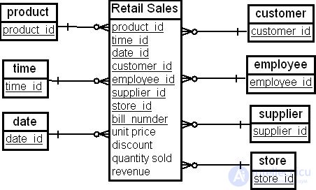
There are two different definitions of fact granularity for the business process defined above. For sales analysis, granularity can be defined as follows (Case 1): each product item included in a single purchase receipt.
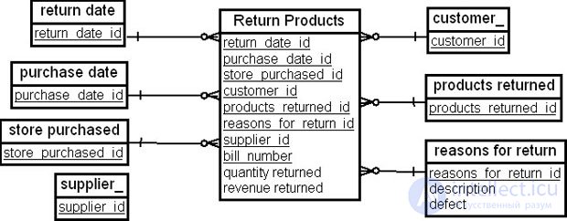
For analyzing the reasons for product returns, granularity can be defined as follows (Case 2): a specific product returned by a customer at any of the stores.
In the first case, the dimensions will be "Product" ( product ), "Time" ( time ), "Customer" ( customer ), "Date" ( date ), "Salesperson" ( employee ), "Supplier" ( supplier ), and "Store" ( store ). The following can be chosen as facts: "Unit Price" ( unit price ), "Discount" ( discount ), "Quantity Sold" ( quantity sold ), and "Revenue" ( revenue ). The star schema with the "Retail Sales" fact table ( Retail Sales ) for this case is shown in fig. 16.11.
In the second case, the dimensions will be "Return Date" ( return date ), "Purchase Date" ( purchase date ), "Customer" ( customer ), "Store that sold the defective product" ( store purchased ), "Returned Product" ( products returned ), "Reason for Return" ( reasons for return ), "Supplier" ( supplier ). The following can be chosen as facts: "Revenue Lost from Returns" ( revenue returned ) and "Quantity Returned" ( quantity returned ). The star schema with the "Return Products" fact table ( Return Products ) for this case is shown in fig. 16.12.
As can be seen from the above, a single business process may correspond to several multidimensional models. The number of fact tables to create for a single business process is determined by the DW designer. It is clear that each business process should have one model (star or snowflake schema). If the granularity of the facts differs, they should be placed in separate tables.
At the next step of transforming the corporate data model into a DW model, the designer merges the set of corporate data model tables into DW tables within the chosen multidimensional model. Corporate data model tables are, as a rule, normalized in accordance with the requirements of the relational model. Merging several normalized tables into one is a denormalization of the database schema. For a large DW, denormalization is performed for performance reasons. Merging tables saves disk space and increases query processing performance.
Despite these performance considerations, when merging tables the DW designer must remember that it makes sense to merge tables if:
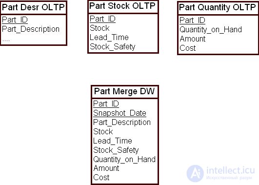
Let us consider the example in fig. 16.13. In the corporate data model there are three normalized tables containing data about products. All three tables of the OLTP system's database, shown at the top of the figure, have the same primary key, "Part Number" ( Part_ID ). Therefore, it makes sense to merge these tables into one, "Parts Merged" ( Part Merge DW ), in the DW model, as shown at the bottom of the figure.
Normalized corporate data model tables do not contain periodic groups and data arrays. These are the requirements of the relational model. However, for a DW, using such data elements may be worthwhile. At their discretion, the DW designer can consider the question of creating data arrays within the relational model. When deciding whether to create data arrays, the following considerations can be used as guidance — it makes sense to create a data array if:
From the standpoint of the physical design of the database schema, this is called splitting or partitioning of tables. Splitting and partitioning are similar techniques but differ in their implementation mechanism. Splitting is a logical technique, while partitioning is a built-in mechanism of the SQL dialect. Partitioning is usually used for a DW.
Partitioning is performed for the sake of improving query processing performance. The rationale for using partitioning in DW schemas, briefly stated, is as follows. There is typically a single fact table. The time attribute is typically part of the key. Time, by its nature, has a predictable measurement structure — day, week, month, quarter, year, and so on. Therefore, it is worth considering partitioning the fact table by units of time.
For example, telephone companies often bill their subscribers for calls made over the course of a month. Therefore, one can consider representing the subscriber billing table as an array of twelve elements, each corresponding to a month of the year. Although in practice the information services of telephone companies rarely use this approach, it turns out to be quite effective from the standpoint of analyzing customer debt.
Examples of table partitioning were discussed in "Introduction to the CASE Tool".
The relational model (and, consequently, the corporate data model built on its basis as well) does not distinguish the rate of data change within a table. One of the main functions of a DW is data accumulation, and the rate of data arrival matters for it. In other words, DWs are sensitive to the rate at which data is added.
To offset the sensitivity to the rate of data addition in a DW, tables should be organized as follows: slowly changing data should be placed in one table, and rapidly changing data in another. That is, the rate of change in the amount of data in each of the DW's tables should be approximately the same.
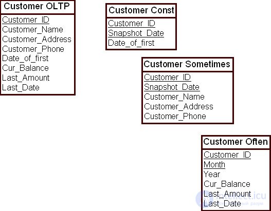
Let us consider an example. The corporate data model contains customer data that has been merged into a single table — "Customers OLTP" ( Customer OLTP ). Among the attributes of this table there is data that never changes, for example, the value of the "First Purchase Date" attribute ( First_Date ). There is also data that sometimes changes, for example, the value of the "Customer Phone" attribute ( Customer_Phone ). There is also data here that changes frequently, for example, the value of the "Last Purchase Date" attribute ( Last_Date ).
It makes sense to split such a table into three tables. The first table contains attributes with constant data; the second contains attributes whose values sometimes change; the third contains attributes whose values change frequently. Fig. 16.14 shows a DW schema that takes into account the principle of attribute value volatility.
Thus, we have examined all eight steps of the basic algorithm for transforming corporate model data into a DW model.
The first stage of the algorithm builds a bridge from the corporate data model to the DW model. Stages two through six essentially represent the multidimensional design process, which we will next examine from the standpoint of using CASE tools for designing multidimensional models. The seventh and eighth steps are directly related to ensuring DW performance at the level of design decisions.
We will examine the application of CASE tools using the example of the PowerDesigner product from Sybase for modeling a DW based on Microsoft's MS SQL Server DBMS.
Suppose that the management of a publishing-industry retail company has decided to implement a DW (specifically, a data mart) for analyzing publication sales and analyzing authors' contributions to the company's total revenue. By the time the decision was made to develop the data mart, the company's IT department already had a corporate data model and an operational data processing system running on MS SQL Server.
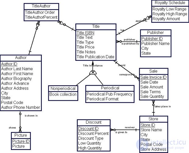
The logical schema of the publishing company's corporate model is shown in fig. 16.15.
The company's corporate data model is documented. All entities, entity attributes, and domains are described. An example description of the "Author" ( Autor ) entity is given in Table 16.1.
| Attribute Name | Attribute Code | Data Type | Domain | Key | |
|---|---|---|---|---|---|
| 1 | Author ID (Идентификатор автора) | AU_ID | A12 | Alphanumeric | Yes, NOT NULL |
| 2 | Author Last Name (Фамилия) | AU_LNAME | VA40 | Alphabetic | NOT NULL |
| 3 | Author First Name (Имя) | AU_FNAME | VA40 | Alphabetic | NOT NULL |
| 4 | Author Biography (Биография автора) | AUTHOR BIOGRAPHY | TXT | Text | |
| 5 | Author Advance (Доплаты авторам) | AU_ADVANCE | MN8,2 | Decimal number | |
| 6 | Author Address (Адрес автора) | AU_ADDRESS | VA80 | Text | |
| 7 | City (Населенный пункт) | CITY | VA20 | Alphabetic | |
| 8 | State (Область) | STATE | VA80 | Alphabetic | |
| 9 | Postal Code (Почтовый индекс) | POSTALCODE | N | Integer | |
| 10 | Author Phone Number (Телефон автора) | AU_PHONE | A12 | Alphanumeric | NOT NULL |
Let us identify the business processes of the data mart's subject area based on the entity-relationship model shown in Fig. 16.15, and apply the corporate model transformation algorithm described in the previous sections of this lecture.
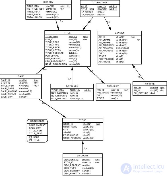
To design the multidimensional model, we will also need another document – the physical model of the company's operational data processing system, shown in Fig. 16.16.
We need it to correctly choose the field names and their types when transferring them into the multidimensional data model.
From the tasks set by the management of the publishing retail company, it follows that we have two business processes for the data warehouse model: sales of publications through stores, and sales of publications by specific authors.
For the business process of selling publications through stores (business process 1), we have the following entities of the corporate data model:
For the business process of selling publications by a specific author (business process 2), we have the following entities of the corporate data model:
We will examine the application of the algorithm for transforming the corporate model into a multidimensional data model using business process 1 as an example. The transformation for business process 2 is performed in the same way.
Note that facts in a multidimensional model reflect "many-to-many" relationships between dimensions. This means that foreign keys in fact tables should be sought in the relations that resolve such relationships.
It is good practice to split the selected entities into two classes: transactional entities, which record business operations, and non-transactional entities, which store descriptions of business operations and business processes. The former are candidates for fact table prototypes, while the latter are candidates for dimension table prototypes of the multidimensional model.
For business process 1, this split is shown in Table 11.2.
| Transactional entities | Non-transactional entities |
|---|---|
| "Sale" (Sale) - describes the business operation of selling a publication | "Store" (Store) describes the store as a business process object through which the sale is carried out |
| "Title" (Тitle) with its subordinate "Periodical" (Periodical) and "Nonperiodical" (Nonperiodical) describes the publications sold in stores |
Thus, for business process 1 we have the fact table "Sale" (Sale) and two dimension tables "Store" (Store) and "Title" (Тitle); note that in the physical model the "Title" entity was denormalized by including the attributes of the subordinate entities "Periodical" ( Periodical ) and "Nonperiodical" ( Nonperiodical ) into it.
Following the corporate model transformation algorithm, let us select the entity attributes that are worth representing in the multidimensional model of the data mart. It is convenient to compile the results into a table, as shown in Table 11.3.
Suppose we are going to create the transactional fact table "Sale" (Sale) for our data mart. Then the time dependency of the data will be determined by the sale date, i.e., by the value of the attribute "Sale Date" ( SALE_DATE ) (the second stage of the corporate data model transformation algorithm). Therefore, we will not introduce any additional timestamps into our multidimensional model, nor will we introduce derived fields (aggregates) into the model.
Let us now consider the relationships between the data (the fourth stage of the corporate data model transformation). In our case of a transactional fact table, no transformation of relationships is required. The fact table records the history of daily sales of publications in stores.
Let us now determine the level of granularity of the facts (the fifth stage of the corporate data model transformation). A specific title is sold in a specific store on a specific day. This business rule determines the granularity level of the facts: the fact table will have one row for each sale, recording the sale of a specific title in a specific store on a specific day.
In our case there are no data arrays, so we will not perform the sixth stage of the transformation algorithm.
Now we have the data we need to build the multidimensional data model. Let us choose a star schema for our multidimensional model.
Partitioning of the fact tables will be discussed later, after building the multidimensional model.
Let us consider using the corporate data model transformation algorithm with the help of Sybase's PowerDesigner CASE tool.
First we will create a multidimensional model of a data mart for analyzing publication sales.
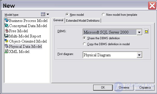
To do this, let us launch the PowerDesigner CASE tool and select the function " Create a new physical data model " (menu items File  New ). In the " New " dialog box that appears on the screen, select the item "Physical Data Model" ( Physical Data Model ) in the "Model type" ( Model type ) list, select MS SQL Server from the DBMS ( DBMS ) drop-down list, and select "Physical Diagram" ( Physical Diagram ) from the "First Diagram" ( First Diagram ) list, then click the " OK " button ( Fig. 16.17).
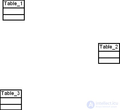
Next we will create the tables that will serve as the fact table and the two dimension tables, using the tool palette ( Palette ). To create a table, you need to move the mouse cursor to the table icon on the tool palette, click on the icon with the left mouse button, move the cursor to the workspace, click the left mouse button again ( Fig. 16.18), and select the pointer icon on the tool palette to move on to other functions.
Now let us transfer the data from the tables of the corporate data model into the objects of the multidimensional data model (i.e., let us perform the sixth stage of the corporate data model transformation algorithm).
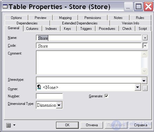
Let us start by defining the elements of the dimension tables. As an example, consider the "Store" ( Store ) dimension. Double-clicking with the mouse on the table diagram opens the "Table Properties … " dialog box, and in the "Name" ( Name ) field of the "General" ( General ) tab we type " Store ". Next, in the "Dimensional Type" ( Dimensional Type ) list, select the table type "Dimension" ( Dimension ) and click the " Apply " button ( Fig. 16.19).
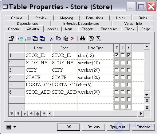
Now let us go to the "Columns" ( Columns ) tab. In the table that opens, we type in the names of the dimension's attributes (see Table 11.3 and Fig. 16.20), set the STOR_ID column as the dimension's primary key, and click the " OK " button.
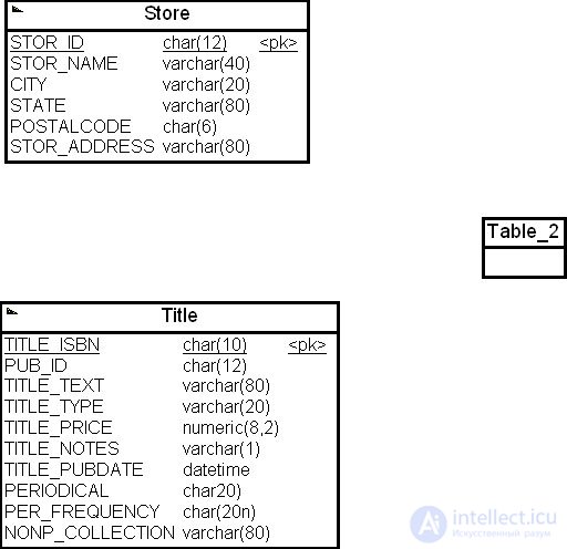
Performing similar operations for the "Title" ( Title ) dimension with the primary key TITLE_ISBN, we obtain the schema fragment shown in Fig. 16.21.
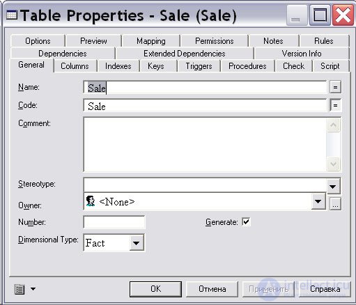
Now let us move on to defining the fields of the fact table. Double-clicking with the mouse on the table diagram opens the "Table Properties …" dialog box, and in the "Name" ( Name ) field of the "General" ( General ) tab we type " Sale ". Next, in the "Dimensional Type" ( Dimensional Type ) list, select the table type "Fact" ( Fact ) and click the " Apply " button ( Fig. 16.22).
Next let us go to the "Columns" ( Columns ) tab. In the table that opens, we type in the names of the fact's attributes and metrics (see Table 11.3 and Fig. 16.20) and click the " OK " button ( Fig. 16.23).
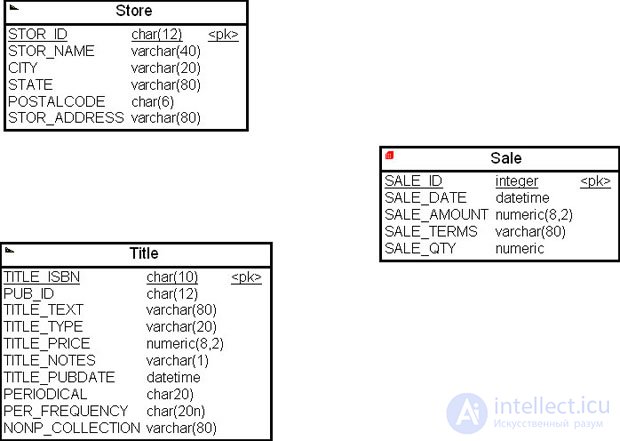
The field SALE_ID is chosen as the primary key of the fact table. Now let us move on to establishing the relationships between the fact table and the dimension tables, i.e., let us reflect in the multidimensional model the results of the fourth and fifth stages of the corporate data model transformation algorithm.
In order to establish a relationship between the tables, you need to move the mouse cursor to the relationship icon on the tool palette, click it with the left mouse button, position the mouse cursor over a table (in our case — the fact table), and, without releasing the left mouse button, drag the cursor to another table (in our case, a dimension table) and release the mouse button ( Fig. 16.24).
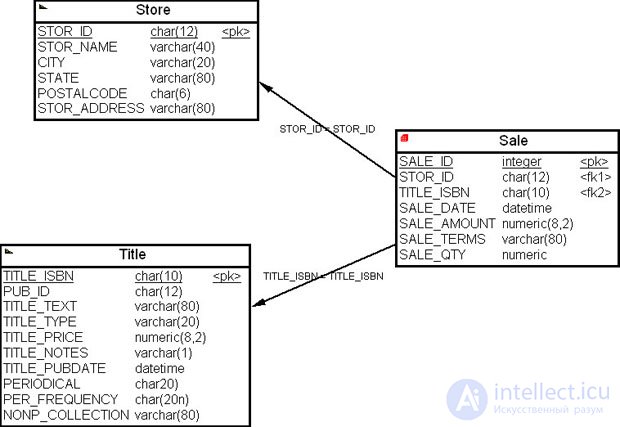
The relationship between the tables is shown on the diagram as an arrow, which in this case is labeled with the join condition of the tables. The primary keys of the dimensions will appear in the fact table as foreign keys of the fact table.
Thus, we have completed building the multidimensional model of the data mart based on the corporate data model.
The script for creating the data mart in MS SQL Server is given below.
/* Table: Sale                                                  */
create table Sale (
   SALE_ID              integer              not null,
   STOR_ID              char(12)             null,
   TITLE_ISBN           char(10)             null,
   SALE_DATE            datetime             null,
   SALE_AMOUNT          numeric(8,2)         null,
   SALE_TERMS           varchar(80)          null,
   SALE_QTY             numeric              null,
   constraint PK_SALE primary key  (SALE_ID)
)
go

/* Table: Store                                                 */
create table Store (
   STOR_ID              char(12)             not null,
   STOR_NAME            varchar(40)          null,
   CITY                 varchar(20)          null,
   STATE                varchar(80)          null,
   POSTALCODE           char(6)              null,
   STOR_ADDRESS         varchar(80)          null,
   constraint PK_STORE primary key (STOR_ID)
)
go

/* Table: Title                                                 */
create table Title (
   TITLE_ISBN           char(10)             not null,
   PUB_ID               char(12)             null,
   TITLE_TEXT           varchar(80)          null,
   TITLE_TYPE           varchar(20)          null,
   TITLE_PRICE          numeric(8,2)         null,
   TITLE_NOTES          varchar(1)           null,
   TITLE_PUBDATE        datetime             null,
   PERIODICAL           char20)              null,
   PER_FREQUENCY        char(20n)            null,
   NONP_COLLECTION      varchar(80)          null,
   constraint PK_TITLE primary key  (TITLE_ISBN)
)
go

alter table Sale
   add constraint FK_SALE_REFERENCE_STORE foreign key (STOR_ID)
      references Store (STOR_ID)
go

alter table Sale
   add constraint FK_SALE_REFERENCE_TITLE foreign key (TITLE_ISBN)
      references Title (TITLE_ISBN)
go
Listing .The data mart we built is intended for analyzing the sales of a publishing retail company through its network of stores (business process 1).
By carrying out similar reasoning for business process 2, we obtain a multidimensional model schema consisting of the fact table "Sales by Author" ( Sale_Author ) and the dimension "Authors" ( Author ), as shown in Fig. 16.25.
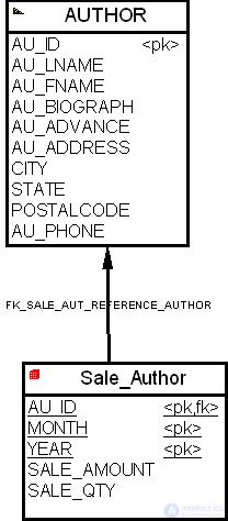
Note that in this multidimensional model of the data mart, the granularity is defined as sales by author per month, and the fact table fields "Sale Amount" ( SALE_AMOUNT ) and "Sale Quantity" ( SALE_QTY ) are derived fields, computed as the corresponding sums for the month.
Let us look at how CASE tools help the data designer perform partitioning of tables in the multidimensional data model. Let us return to the example from the previous section of this lecture and consider the multidimensional model of the data mart in Fig. 16.24.
Suppose the marketing department constantly analyzes sales of publications for the current year, while sales analysis by year is performed once a year. In that case, in order to increase query performance, it makes sense to perform horizontal partitioning of the "Sale" ( Sale ) fact table by year. To do this, let us introduce the attribute "Sale Year" ( SALE_YEAR ) into the fact table ( Fig. 16.26). Let us also assume that the data mart will be populated with data starting from 2007.
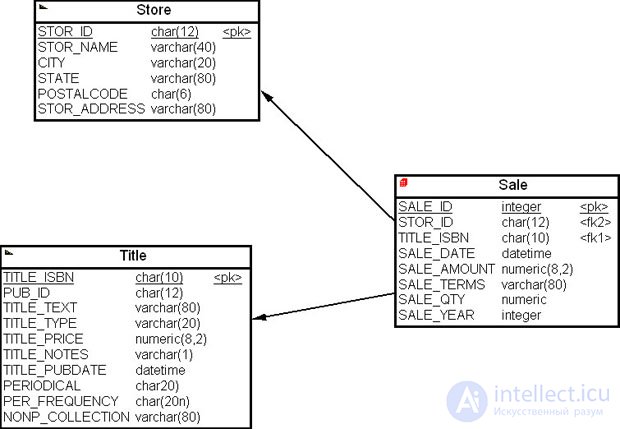
Note that instead of this step, we could have introduced another dimension table "Time" with a "Year" attribute and established a relationship between this dimension and the model's fact table.
Recall that horizontal partitioning of a table consists of splitting the original table into several tables, each of which contains a subset of the rows of the original table.
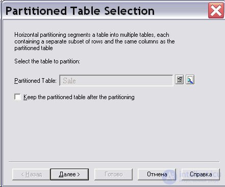
To perform horizontal partitioning of the "Sale" ( Sale ) fact table using PowerDesigner CASE, you can right-click on the fact table and select "Horizontal Partitioning" ( Horizontal Partitioning ) from the pop-up menu. The "Partitioned Table Selection" ( Partitioned Table Selection ) dialog box will appear on the screen. After selecting the "Sale" ( Sale ) table, click the " Next " button ( Fig. 16.27).
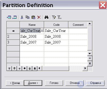
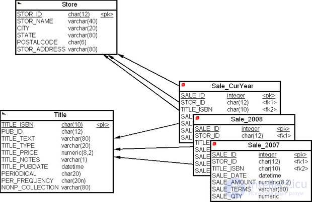
The "Partition Definitions" ( Partition Definitions ) dialog box will appear on the screen, in which you need to define the partition names (let these be the names Sale_CurYear, Sale_2008, and Sale_2007 ) and click the " Next " button ( Fig. 16.28).
The "Discriminant Column Selection" ( Discriminant Column Selection ) dialog box will appear on the screen. The discriminant column is a table column that is part of the partitioning criterion, so it does not have to be stored in the partitions. By left-clicking on the " Add Row " icon, you activate the "Selection" ( Selection ) dialog box. Let us select from the list of columns the "Sale Year" ( SALE_YEAR ) column, by which the partitioning will be performed, and click the " OK " and " Next " buttons ( Fig. 16.29).
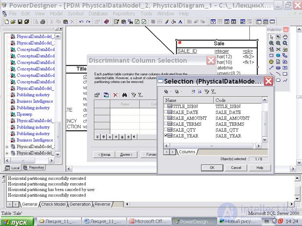
The "Partitioning Information" ( Partitioning Information ) dialog box will appear on the screen. Next, let us click the " Finish " button. After arranging the partitions in the workspace, we obtain the multidimensional data model of our data mart with the partitioned "Sale" ( Sale ) table, as shown in Fig. 16.30.
Thus, using an example, we have reviewed how a CASE tool can be used to transform a corporate data model into a multidimensional data warehouse model.
When building an enterprise-wide data warehouse, the corporate data model, as a rule, serves as the starting point for designing the data warehouse model. In this case, the data warehouse model design procedure can be broken down into the following steps.
From the standpoint of a particular SQL dialect, a few more steps can be added to the algorithm considered, also related to ensuring data warehouse performance at the design level — in particular, dimension hierarchies and materialized views.
It is advisable to design a data warehouse model based on an organization's corporate data model with the help of CASE tools. Using CASE tools increases the productivity of the data warehouse designer, especially for large and medium-sized projects.

Comments