
Lecture
OLAP technology is not a specific software product, nor a programming language. If we try to encompass OLAP in all its manifestations, it is a collection of concepts, principles, and requirements underlying software products that make data access easier for analysts.
Analysts are the primary consumers of corporate information. An analyst's task is to find patterns in large volumes of data. Therefore, an analyst is not interested in an isolated fact, such as that on a certain day a batch of ballpoint pens was sold to customer Ivanov — they need information about hundreds and thousands of similar events. Individual facts in a data warehouse might interest, for example, an accountant or a sales department manager responsible for a specific contract. A single record is not enough for an analyst — they might, for instance, need information about all the contracts of a sales point for a month, quarter, or year. An analyst may not be interested in a customer's tax ID or phone number — they work with concrete numerical data, which constitutes the essence of their professional activity.
Centralization and convenient structuring are far from all an analyst needs. They also need a tool for viewing and visualizing information. Traditional reports, even those built on a unified data warehouse, nevertheless lack a certain flexibility. You cannot "rotate," "expand," or "collapse" them to get the required view of the data. The more "slices" and "cuts" of data an analyst can explore, the more ideas they generate, which in turn require ever more "slices" to verify. OLAP serves as exactly this kind of tool for an analyst's data exploration.
Although OLAP is not a mandatory attribute of a data warehouse, it is increasingly used to analyze the information accumulated in that warehouse.
Operational data is collected from various sources, cleaned, integrated, and stored in the data warehouse. At that point it is already available for analysis using various reporting tools. The data (fully or partially) is then prepared for OLAP analysis. It may be loaded into a dedicated OLAP database or left in the relational data warehouse. A crucial element of OLAP usage is metadata, i.e., information about the structure, placement, and transformation of the data. Metadata is what ensures the effective interaction of the various components of the warehouse.
Thus, OLAP can be defined as a collection of tools for multidimensional analysis of data accumulated in a data warehouse. In theory, OLAP tools can be applied directly to operational data or exact copies of it. However, doing so carries the risk of analyzing data that is not actually suitable for such analysis.
Multidimensional data analysis is the foundation of OLAP. It can be performed using various tools, which can conventionally be divided into client-side and server-side OLAP tools.
Client-side OLAP tools are applications that compute aggregate data (sums, averages, maximum or minimum values) and display it, with the aggregate data itself held in a cache within that OLAP tool's own address space.
If the source data resides in a desktop DBMS, the aggregate data is computed by the OLAP tool itself. If instead the source data comes from a server DBMS, many client-side OLAP tools send SQL queries containing a GROUP BY clause to the server, and receive back the aggregate data computed on the server.
As a rule, OLAP functionality is implemented in statistical data processing tools (products from Stat Soft and SPSS are widely used in this class on the Russian market) and in some spreadsheet applications. In particular, Microsoft Excel 2000 has quite good multidimensional analysis capabilities. With this product you can create and save a small local multidimensional OLAP cube as a file and display its two- or three-dimensional cross-sections.
Many development tools contain class libraries or components that let you build applications implementing basic OLAP functionality (such as the Decision Cube components in Borland Delphi and Borland C++Builder). In addition, many companies offer ActiveX controls and other libraries that implement similar functionality.
Note that client-side OLAP tools are typically used with a small number of dimensions (usually no more than six is recommended) and a small variety of values for these parameters — since the resulting aggregate data must fit within that tool's address space, and its volume grows exponentially as the number of dimensions increases. That is why even the most basic client-side OLAP tools usually let you pre-calculate the amount of RAM required to build a multidimensional cube in memory.
Many (though not all) client-side OLAP tools allow the contents of the aggregate-data cache to be saved as a file, which in turn avoids the need to recompute them. Note that this capability is often used to extract aggregate data for the purpose of transferring it to other organizations or for publication. A typical example of such extractable aggregate data is morbidity statistics broken down by region and age group, which is open information published by health ministries of various countries and the World Health Organization. Meanwhile, the actual source data — records of specific illness cases — is confidential information belonging to medical institutions and must never fall into the hands of insurance companies, let alone become public knowledge.
The idea of saving the aggregate-data cache to a file was further developed in server-side OLAP tools, where the storage and modification of aggregate data, as well as maintenance of the repository holding it, are carried out by a separate application or process called an OLAP server. Client applications can query such a multidimensional repository and receive data in response. Some client applications can also create such repositories or update them to reflect changed source data.
The advantages of server-side OLAP tools over client-side OLAP tools are similar to the advantages of server DBMSs over desktop ones: when server-side tools are used, the computation and storage of aggregate data takes place on the server, and the client application only receives the results of queries against it, which generally reduces network traffic, query execution time, and the resource requirements placed on the client application. Note that enterprise-scale data analysis and processing tools are typically based on server-side OLAP tools, such as Oracle Express Server, Microsoft SQL Server 2000 Analysis Services, Hyperion Essbase, and products from Crystal Decisions, Business Objects, Cognos, and SAS Institute. Since all the leading server DBMS vendors produce (or have licensed from other companies) some server-side OLAP tool, the selection is fairly wide, and in almost every case you can obtain an OLAP server from the same vendor as your database server.
Note that many client-side OLAP tools (in particular, Microsoft Excel 2003, Seagate Analysis, and others) can connect to server-side OLAP repositories, acting in that case as client applications performing such queries. In addition, there are quite a few products that serve as client applications for OLAP tools from various vendors.
Multidimensional data warehouses contain aggregate data at various levels of detail, for example, sales volumes by day, month, year, and product category, etc. The purpose of storing aggregate data is to reduce query execution time, since in most cases it is summary rather than detailed data that is of interest for analysis and forecasting. That is why, when a multidimensional database is created, certain aggregate data is always computed and stored.
Note that storing all aggregate data is not always justified. The reason is that as new dimensions are added, the volume of data making up the cube grows exponentially (sometimes referred to as "explosive growth" of data volume). More precisely, the rate of growth of aggregate data volume depends on the number of dimensions in the cube and the number of members at the various hierarchy levels of those dimensions. To address the "explosive growth" problem, various schemes are used that achieve acceptable query performance without computing anywhere near all possible aggregate data.
Both source and aggregate data can be stored either in relational or in multidimensional structures. As a result, three data storage approaches are currently in use.
Some OLAP tools support storing data only in relational structures, while others support only multidimensional storage. However, most modern server-side OLAP tools support all three storage approaches. The choice of storage approach depends on the volume and structure of the source data, the required query performance, and the frequency with which the OLAP cubes must be refreshed.
Note also that the vast majority of modern OLAP tools do not store "empty" values (an example of an "empty" value would be the absence of sales of a seasonal product outside its season).
The technology of comprehensive multidimensional data analysis is known as OLAP (On-Line Analytical Processing). OLAP is a key component of data warehouse organization. The OLAP concept was described in 1993 by Edgar Codd, a well-known database researcher and the author of the relational data model. In 1995, based on the requirements set out by Codd, the so-called FASMI test (Fast Analysis of Shared Multidimensional Information) was formulated — a fast analysis of shared multidimensional information, comprising the following requirements for multidimensional analysis applications:
It should be noted that OLAP functionality can be implemented in various ways, ranging from the simplest data analysis tools in office applications to distributed analytical systems built on server products.
OLAP provides convenient, high-performance tools for accessing, viewing, and analyzing business information. The user gets a natural, intuitive data model, organizing data as multidimensional cubes. The axes of the multidimensional coordinate system are the main attributes of the business process being analyzed. For sales, for example, these might be product, region, and customer type. Time is used as one of the dimensions. At the intersections of the dimension axes lie the data that quantitatively characterize the process — measures. These might be sales volumes in units or monetary terms, warehouse stock, costs, and so on. A user analyzing the information can "slice" the cube along different directions, obtaining summary information (for example, by year) or, conversely, detailed information (by week), and perform whatever other manipulations occur to them during the analysis process.
In the three-dimensional cube shown in Fig. 26.1, sales totals are used as the measure, while time, product, and store are used as dimensions. The dimensions are shown at particular grouping levels: products are grouped by category, stores by country, and transaction time data by month. We will look at grouping levels (hierarchies) in more detail shortly.
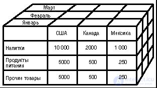
Even a three-dimensional cube is difficult to display on a computer screen in a way that shows the values of the measures of interest. This is even more true for cubes with more than three dimensions. To visualize data stored in a cube, the familiar two-dimensional, i.e., tabular, representations are typically used, with complex hierarchical row and column headers.
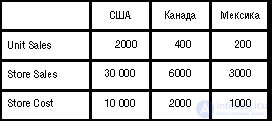
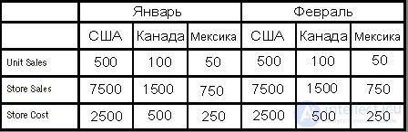
A two-dimensional view of a cube can be obtained by "slicing" it across one or more axes (dimensions): we fix the values of all dimensions except two — and get an ordinary two-dimensional table. One dimension is represented along the horizontal axis of the table (column headers), another along the vertical axis (row headers), and the cells of the table hold the measure values. In this case the set of measures is effectively treated as one of the dimensions: we either choose a single measure to display (in which case we can place two dimensions in the row and column headers), or we show several measures (in which case one of the table's axes is occupied by the measure names, and the other by the values of the single "unsliced" dimension).
Take a look at Fig. 26.2. It shows a two-dimensional slice of the cube for a single measure — Unit Sales — and two "unsliced" dimensions — Store and Time.
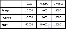
Fig. 26.3 shows only one "unsliced" dimension — Store — but displays the values of several measures — Unit Sales, Store Sales, and Store Cost.
A two-dimensional view of the cube is also possible when more than two dimensions remain "unsliced." In that case, two or more dimensions of the "sliced" cube are placed on the axes of the slice (rows and columns) — see Fig. 26.4.
The values "plotted" along the dimensions are called members or labels (members). Labels are used both for "slicing" the cube and for restricting (filtering) the selected data — when for a dimension that remains "unsliced" we are interested not in all values but in a subset of them, for example, three cities out of several dozen. Label values are displayed in the two-dimensional view of the cube as row and column headers.
Labels can be combined into hierarchies, consisting of one or more levels. For example, the labels of the "Store" dimension naturally combine into a hierarchy with the following levels:
| All (World) |
| Country |
| State |
| City |
| Store. |
Aggregate values are computed according to hierarchy levels, for example, sales volume for the USA (the "Country" level) or for the state of California (the "State" level). More than one hierarchy can be implemented for a single dimension — for instance, for time: {Year, Quarter, Month, Day} and {Year, Week, Day}.
Note that hierarchies can be balanced, such as the hierarchy shown in Fig. 26.5, as well as hierarchies based on date-time data, or unbalanced. A typical example of an unbalanced hierarchy is a "manager-subordinate" type hierarchy (which can be built, for example, using the values of the Salesperson field from the sample dataset discussed above), as shown in Fig. 26.6.
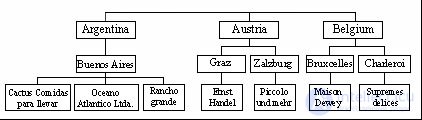
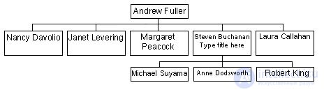
Such hierarchies are sometimes referred to as parent-child hierarchies.
There are also hierarchies that occupy an intermediate position between balanced and unbalanced (referred to as "ragged"). They usually contain members whose logical "parents" are not located directly at the level immediately above (for example, a geographic hierarchy has the levels Country, City, and State, but the dataset includes countries that have no states or regions between the Country and City levels (Fig. 26.7)).
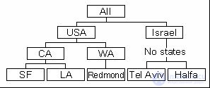
Note that not every OLAP tool supports unbalanced and "ragged" hierarchies. For example, Microsoft Analysis Services 2000 supports both hierarchy types, while Microsoft OLAP Services 7.0 supports only balanced ones. Different OLAP tools may also differ in the number of hierarchy levels, the maximum number of members allowed at a single level, and the maximum possible number of dimensions themselves.
Everything said above about OLAP essentially concerned the multidimensional representation of data. How the data is actually stored, roughly speaking, does not concern either the end user or the developers of the tool the client uses.
Multidimensionality in OLAP applications can be divided into three levels.
The first two levels are mandatory in all OLAP tools. The third level, although widespread, is not mandatory, since the data for the multidimensional representation can also be extracted from ordinary relational structures; in that case, the multidimensional query processor translates multidimensional queries into SQL queries that are executed by the relational DBMS.
Specific OLAP products, as a rule, are either a multidimensional data presentation tool (an OLAP client — for example, Pivot Tables in Microsoft Excel 2000 or ProClarity by Knosys), or a multidimensional server DBMS (an OLAP server — for example, Oracle Express Server or Microsoft OLAP Services).
The multidimensional processing layer is typically built into the OLAP client and/or OLAP server, but it can also be provided as a separate component, such as Microsoft's Pivot Table Service.
Let's examine the methodology for designing data cubes for OLAP data warehouses using Sybase's PowerDesigner CASE tool. Note that in presenting this material we will omit many details, leaving them for independent study within the specific CASE tool environment. Our goal is to illustrate the key points of the design methodology and the capabilities of CASE tools for designing multidimensional data schemas.
A multidimensional diagram is a model of an organization's business activity in terms of data cubes and dimensions. In such a diagram, data about the organization's business activity is represented in one of two categories. Numeric data, or metrics, such as the number of sales, are facts of business activity. Representing business activity in terms of geography, products, and time constitutes the dimensions.
A multidimensional diagram is the primary tool used by the designer of an OLAP data warehouse.
OLAP warehouses are populated with data from a data warehouse or data marts. This data transfer is carried out by mapping the relational representation to the multidimensional data representation. Thus, data warehouses act as the data source for OLAP warehouses.
The primary users of such OLAP data warehouses are business analysts. Analysts query OLAP warehouses to extract business information. That is why data cubes are designed to support analytical queries and are built according to user-defined dimensions.
Multidimensional analytical queries typically involve calculations, such as computing growth or decline rates, analyzing time series data, and so on. Such queries aim to identify trends in the data and hidden relationships between data items.
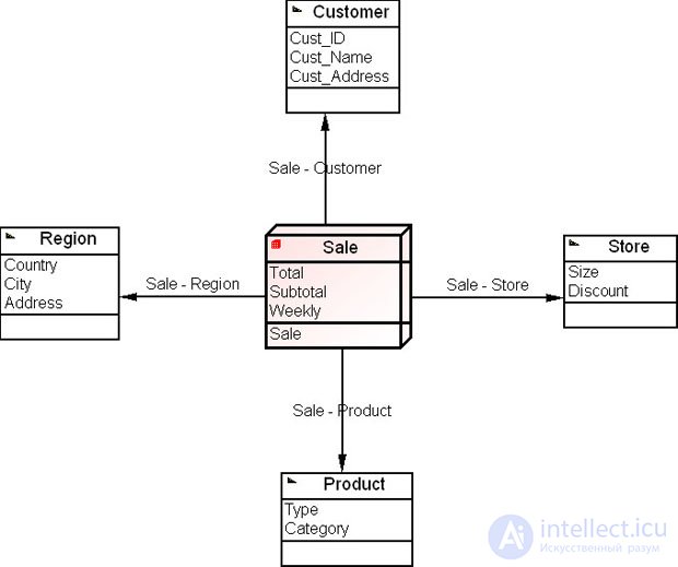
Fig. 26.8 shows an example of a multidimensional diagram. As the figure shows, sales data has the dimensions "Product," "Region," "Customer," and "Store." Facts, such as sales totals, are examined from the perspective of these user-defined dimensions. When an analyst retrieves sales totals for a specific product in a specific region, they are examining the sales data from the perspective of the "Product" and "Region" dimensions. The most commonly used dimension is time, since the main purpose of running analytical queries is to find trends in the data.
The main elements of a multidimensional diagram are:
Only data cubes, dimensions, and associations are represented in the CASE tool palette.
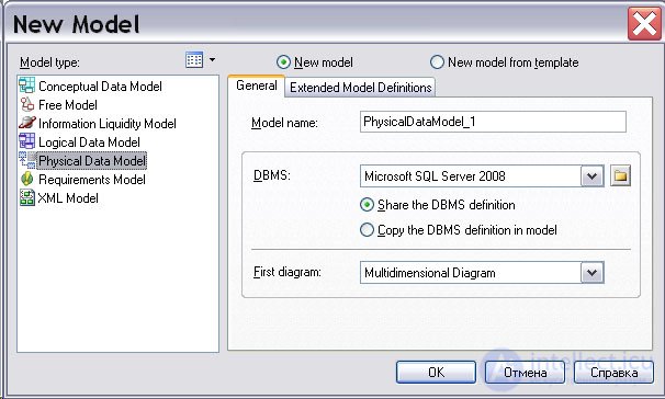
A multidimensional diagram is created as follows. Choose File->New Model from the menu (the "New Model" dialog will appear in the workspace, Fig. 26.9). In this dialog, select the model type "physical data model", choose MS SQL Server as the DBMS from the DBMS drop-down list, specify a multidimensional diagram as the physical model class, assign a name to the multidimensional model (PhysicalDataModel_1), and click the "OK" button.
The multidimensional model has now been created, and the workspace and tool palette are available (Fig. 26.10).
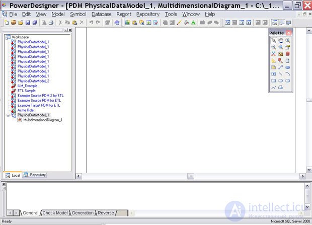
The data warehouse designer can set model properties in the Tools menu item.
Let's take a closer look at building the model's elements.
As mentioned above, a data cube is a set of metrics whose corresponding value is stored in each of its data cells. Metrics are organized according to dimensions in order to support fast data retrieval or drill-down/roll-up operations (drill-down).
As a rule, data cubes are associated with facts, which allow the metrics for the cube to be defined. In a multidimensional diagram, data cubes represent OLAP cubes.
You can use the tool palette to build a data cube. Select the cube icon on the palette and click the left mouse button on the workspace to create a data cube.
Then double-click the data cube to open the dialog box for defining the data cube's properties (Fig. 26.11).
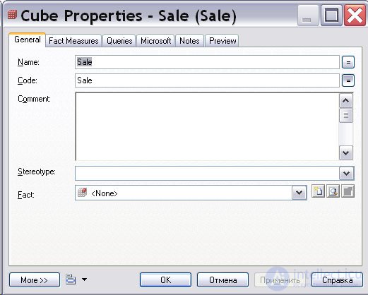
The following properties can be defined for a data cube.
Additional properties of a data cube are:
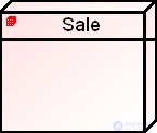
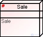
Let's name the data cube "Sale". Fig. 26.12 shows the result of building the data cube in the multidimensional model.
Dimensions are the axes used for analyzing data in a multidimensional data structure.
A dimension consists of an ordered list of attributes that jointly define a common semantic meaning (through their values) in the modeled subject area. Each attribute defines a single position along the axis of the data cube.
Dimensions can be mapped to tables and views, which allows data to be transferred into them from operational systems' databases.
Dimensions can have several hierarchies defined over their set of attributes.
You can use the tool palette to build a dimension. Select the dimension icon on the palette and click the left mouse button on the workspace to create a dimension.
Then double-click the dimension to open the dialog box for defining the dimension's properties (Fig. 26.13).
Let's name the dimension "Time".
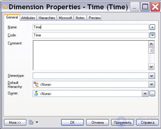
The following properties can be defined for a dimension.
Defining a dimension also includes the following additional properties.
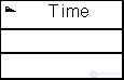
Attributes are qualifiers of dimensions in queries. For example, the "Time" dimension might contain the attributes "Year," "Quarter," "Month," "Week." Attributes can be organized into hierarchies.
Dimension attributes have the following properties.
Additional properties of attributes are:
The dimension properties dialog can be used to create dimension attributes. For example, for the "Time" dimension let us define the following attributes: "Year", "Quarter", "Month" and "Week" – as shown in Fig. 26.15.
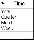
An attribute can participate in the definition of another attribute, thereby complementing that attribute's definition. Such refining attributes are found in the dimension's attribute list and can be used in the definition of another attribute.
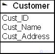
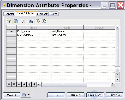
For example, in the "Customer" dimension, the attributes "Cust_Name" and "Cust_Address" can be used to detail the "Cust_ID" attribute ( Fig. 26.16).
To do this, in the dimension properties dialog you need to select the attribute list, choose the Cust_ID attribute in the attribute list, open the attribute properties dialog for it, select the "Detail Attributes" tab in it, and add the Cust_Name and Cust_Address attributes to it, as shown in Fig. 26.17.
A fact corresponds to the focus of the data analysis that supports the organization's management decision-making. A fact is a set of metrics of a data cube. For example, in our example the facts could be "Sale" or revenue and budget. The same facts can be used in various data cubes.
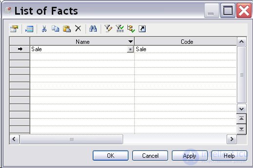
A fact is added to the multidimensional diagram as follows. Select the menu item Model-> Facts and add it to the list in the "List of Facts" dialog box that appears ( List of Facts ), as shown in Fig. 26.18 and Fig. 26.19.
A fact has the following properties.
Additional properties of a fact are:
A measure is a variable that corresponds to the focus of the data analysis. A measure describes the value of a data cube cell. For example, a measure is often the price of a product or a total value. Measures can be the result of calculations.
A measure has the following properties.
Additional properties of a measure are:
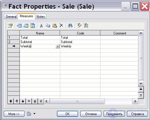
To create a measure, from the main menu Model->Facts in the "List of Facts" dialog box ( List of Facts ) select a fact (in our case Sale) and open the "Fact Properties" dialog box ( Fact Properties ), in which, on the "Measure" tab ( Measure ), add the required measures. In our example let us add the following measures: "Total", "Subtotal" and "Weekly" – as shown in Fig. 26.20.
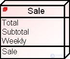
Now the data cube of our example looks as shown in Fig. 26.21.
A hierarchy defines one or more access paths to data through a dimension. There are two main types of hierarchies.
A hierarchy has the following properties.
Additional properties of a hierarchy are:
A hierarchy can be added to a dimension by opening the dimension properties window on the "Hierarchies" tab (Hierarchies), as shown in Fig. 26.22.
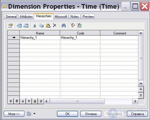
When a hierarchy is created, a default name including a number is assigned. This number is used, by default, when the object is created.
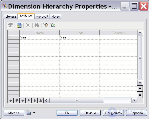
By opening the hierarchy properties dialog box, attributes can be added to the hierarchy, as shown in Fig. 26.23.
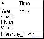
Now on the multidimensional diagram the "Time" dimension looks as shown in Fig. 26.24.
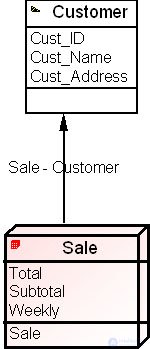
An association links a data cube to the dimension that defines it. An association shows an aspect of the data cube analysis with respect to the specified dimension.
For example, you can link the "Sale" data cube to the "Customer" dimension by means of the "Sale" – "Customer" association (Sale-Customer). Only one association is allowed between a dimension and a data cube.
An association has the following properties.
An association can be created using the tool palette by selecting the association icon. For our example, let us link the "Sale" data cube to the "Customer" dimension, as shown in Fig. 26.25.
Let us add three dimensions to the multidimensional model of our example — "Store", "Region" and "Product". As a result we obtain a multidimensional diagram, as in Fig. 26.8.
However, this is far from everything that still needs to be done to complete the model. The resulting graphical representation of the multidimensional diagram is, for now, practically useless. Let us look at some of the issues that need to be resolved to complete the construction of the multidimensional diagram.
Data cubes in an OLAP data warehouse must be populated with data from the data warehouse, data marts, or the databases of the organization's operational systems (data sources). We must, as they say, populate the data cube.
On the multidimensional diagram, each data cube is linked to a query. For each cube there exists a single mapping to a single data source. The query defined on the cube is used to extract data from the source and then store it in the OLAP warehouse's cube. This link between the data source and the data cube is called mapping a relational schema to a multidimensional one.
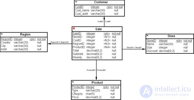
Before proceeding to generate the script for creating a data cube, it needs to be linked to a source, i.e. a mapping from the relational schema to the multidimensional one must be built. To solve this task a data source is required.
Let us assume that for our example the data source is a data mart with the schema shown in Fig. 26.26.
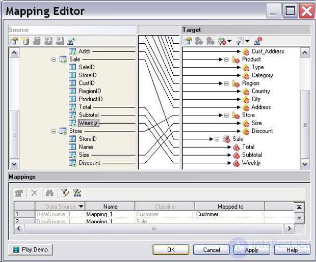
To build the mapping, PowerDesigner provides the Mapping Editor, which is invoked from the menu item Tools->Mapping Editor.
Let us define the data source name as DataSource_1 and bind it to the schema shown in Fig. 26.26, performing the actions prescribed by PowerDesigner. Next we establish links between the fields of the source's fact and dimension tables and the measures, attributes of the data cube, and dimensions of the multidimensional diagram, as shown in Fig. 26.27.
After performing the actions described above, in the "Sale" ( Sale ) data cube properties dialog box, on the Queries tab, you can view the query that will be used to extract data from the source in order to load it into the cube:
select
      Customer.CustID "Cust_ID",
      Customer.Cust_name "Cust_Name",
      Customer.Cust_addr "Cust_Address",
      Region.Country "Country",
      Region.City "City",
      Region.Addr "Address",
      Store.Size "Size",
      Store.Discount "Discount",
      Product.Type "Type",
      Product.Cftegory "Category",
      Sale.Total "Total",
      Sale.Subtotal "Subtotal",
      Sale.Weekly "Weekly"
from  Customer,
      Region,
      Store,
      Product,
      Sale
where Sale.RegionID = Region.RegionID and
      Sale.CustID = Customer.CustID and
      Sale.StoreID = Store.StoreID and
      Sale.ProductID = Product.ProductID
Also, in the "Sale" ( Sale ) data cube properties dialog box, on the Preview tab, you can view the script that will be used to create the data cube:
CREATE CUBE Sale
(
   DIMENSION Customer,
         LEVEL Cust_ID TYPE Regular,
         LEVEL Cust_Name TYPE Regular,
         LEVEL Cust_Address TYPE Regular,
   DIMENSION Region,
         LEVEL Country TYPE Regular,
         LEVEL City TYPE Regular,
         LEVEL Address TYPE Regular,
   DIMENSION Store,
         LEVEL Size TYPE Regular,
         LEVEL Discount TYPE Regular,
   DIMENSION Product,
         LEVEL Type TYPE Regular,
         LEVEL Category TYPE Regular,
   MEASURE Total,
   MEASURE Subtotal,
   MEASURE Weekly
)
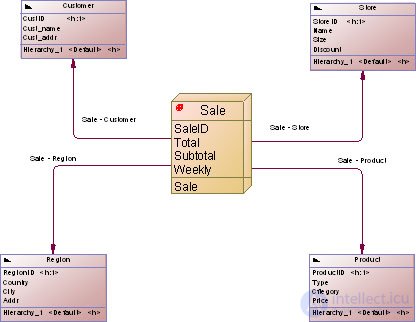
There is a simpler way to create a multidimensional diagram, using the physical data model diagram together with the Rebuild Cubes function, which is invoked from the menu item Tools->Multidimesion->Rebuild Cubes ( Fig. 26.28).
The resulting data cube is shown in Fig. 26.28. As can be seen from the figure, the data cube built this way differs from the one we built in our tutorial example. In this case we did not use the mapping editor directly, so all the fields of the source schema are present in the multidimensional diagram.
Note that in this example the query:
select
      Store.StoreID "StoreID",
      Store.Name "Name",
      Store.Size "Size",
      Store.Discount "Discount",
      Customer.CustID "CustID",
      Customer.Cust_name "Cust_name",
      Customer.Cust_addr "Cust_addr",
      Region.RegionID "RegionID",
      Region.Country "Country",
      Region.City "City",
      Region.Addr "Addr",
      Product.ProductID "ProductID",
      Product.Type "Type",
      Product.Cftegory "Cftegory",
      Product.Price "Price",
      Sale.SaleID "SaleID",
      Sale.Total "Total",
      Sale.Subtotal "Subtotal",
      Sale.Weekly "Weekly"
from  Store,
      Customer,
      Region,
      Product,
      Sale
where Sale.RegionID = Region.RegionID and
      Sale.CustID = Customer.CustID and
      Sale.StoreID = Store.StoreID and
      Sale.ProductID = Product.ProductID
also differs from the one we built earlier. The command for building the data cube also differs:
CREATE CUBE Sale
(
   DIMENSION Store,
         LEVEL StoreID TYPE Regular,
   DIMENSION Customer,
         LEVEL CustID TYPE Regular,
   DIMENSION Region,
         LEVEL RegionID TYPE Regular,
   DIMENSION Product,
         LEVEL ProductID TYPE Regular,
   MEASURE SaleID,
   MEASURE Total,
   MEASURE Subtotal,
   MEASURE Weekly
).
In conclusion, it should be noted that the construction of the multidimensional diagram was illustrative in nature — a number of steps were skipped that would have made the diagram fully functional. Our goal was to demonstrate the methodology for building a multidimensional diagram and to describe the main elements of a multidimensional diagram.
In this work we became acquainted with the basics of OLAP. We learned the following.
In addition, we examined the basic principles of the logical organization of OLAP cubes, and learned the basic terms and concepts used in multidimensional analysis. Finally, we found out what the various types of hierarchies in the dimensions of OLAP cubes represent.
We covered the methodology for building a multidimensional diagram in the CASE tool PowerDesigner and its main elements: data cube, dimension, association, hierarchy, fact, measures, attributes.

Comments